Introduction

Understanding the underlying mechanisms of large language models is critical to mechanistic interpretability research. One of the main challenges is that most neurons and attention heads cannot be independently understood. The field has identified this problem as superposition^[1,2]. This hypothesis suggests that there might exist true features that the model is using to represent information, but these features are often smeared across multiple neurons or attention heads. An active direction in addressing this problem is 1) to find these true features and 2) understand how they interact with each other via model parameters (i.e. circuits).

Sparse dictionary learning methods, particularly sparse autoencoders (SAEs)^[3,4], have emerged as a promising approach to extract monosemantic features from language models. A variant called transcoders^[5,6,7] makes circuit identification easier by approximating MLP outputs with sparse features. Recent work has used transcoders to build attribution graphs (visual representations of how features influence model outputs) for specific prompts^[6,8].

However, these approaches share a critical limitation: §?. Existing methods decompose MLP computation but treat attention patterns as given, leaving attention superposition unresolved. We address this by introducing complete replacement models (CRMs), which combine transcoders for MLPs with Low-Rank Sparse Attention (Lorsa)^[9] modules for attention layers. This gives us interpretable features for every computational block.

Complete replacement models. In §?, we introduce CRMs, which replace each attention and MLP layer with a sparse replacement layer trained to approximate the original layer's output. Each Lorsa feature has its own QK circuit (determining where to attend) and rank-1 OV circuit (determining what to read and write), making attention computation fully decomposable. By freezing attention patterns and layernorm denominators during attribution, we convert the model into a linear computation graph where all feature interactions flow through interpretable virtual weights. This architectural completeness is key to both efficient attribution and global weight analysis.

Why attention matters. Training SAEs on attention outputs can extract monosemantic features^[10,11], but these features may still be collectively computed by multiple heads. This makes it difficult to trace how attention patterns form, a process called §?. Lorsa solves this by decomposing attention into sparse, independently interpretable features, each with its own QK and OV circuits.

Complete attribution graphs. In §?, we show how CRMs convert all attention-mediated paths into combinations of interpretable feature interactions. This eliminates the exponential growth of possible paths between features and enables complete attribution graphs that trace both MLP and attention circuits.

Revisiting the biology of language models. In §?, we apply CRMs to study how Qwen3-1.7B implements specific behaviors. In string indexing tasks, we trace how the model selectively retrieves characters at different positions through shared attention feature families. For induction, we identify distinct subcircuits operating at different depths: lower layers perform relation-keyed binding while higher layers execute generic retrieval. These case studies reveal attention-mediated feature interactions that were previously hidden in transcoder-only analyses.

Global circuits. In §?, we show how architectural completeness unlocks efficient global weight analysis. Because all feature interactions flow through static virtual weights rather than input-dependent attention patterns, we can compute expected attributions over distributions and construct global circuit atlases. These reveal canonical computational patterns such as induction circuits at the feature level for the first time.

Evaluation. In §?, we evaluate our CRMs trained on Qwen3-1.7B in three dimensions: interpretability (feature quality and reconstruction fidelity), sufficiency (how well attribution graphs capture model behavior), and mechanistic faithfulness (whether interventions match predictions). While Lorsa introduces additional reconstruction error, the resulting attribution graphs achieve comparable faithfulness to transcoder-only models while providing complete circuit coverage.

Replacement Layers

Replacement layers are sparse, interpretable modules trained to approximate the computation of individual attention or MLP modules in the underlying model. Each replacement layer learns a dictionary of features and uses sparse coding to reconstruct the original layer's output: sparse codes are computed from the layer inputs, then decoded through the dictionary to approximate the original output. Conceptually, the original layer is "sandwiched" between the encoder (which computes sparse features from inputs) and the decoder (which reconstructs outputs from these features), allowing us to decompose the computation into interpretable, monosemantic components. By combining replacement layers for all underlying layers, we obtain a §? that rewrites the model's computation in a more interpretable form.

Transcoders

Transcoders^[6,7,8] are replacement layers that approximate the computation of an MLP layer. In this work, we use the per-layer version instead of cross-layer transcoders^[8] for both conceptual and engineering simplicity. A Per-layer Transcoder (PLT) has the same architecture as Sparse Autoencoders (SAEs) ^[3,4], but learns to approximate downstream activations instead of its original input.

Concretely, given an MLP input activation, denoted as \mathbf{x} \in \mathbb{R}^d, the transcoder computes the feature activation as:

where \mathbf{W}_\text{enc} \in \mathbb{R}^{F \times d} is the encoder weight matrix. The input is encoded into a feature activation space with F \gg d dimensions, followed by a Top-K sparsity constraint to select the K strongest features and set others to zero^[12]. Alternative sparsity constraints such as BatchTopK^[13] and JumpReLU^[14] should have similar effect^[15].

The sparse feature activations are then decoded to the output space as:

where \mathbf{W}_\text{dec} \in \mathbb{R}^{d \times F} is the decoder weight matrix, and \mathbf{b}_\text{dec} \in \mathbb{R}^d is the decoder bias.

The transcoder is trained to simply minimize the mean squared error between the decoded output and the original output \mathbf{y} \in \mathbb{R}^d:

Low-Rank Sparse Attention (Lorsa)

Lorsa^[9] is designed as a sparse replacement model for attention layers. As the attention counterpart of transcoders, it is also trained to find a sparse representation of the attention layer output, while also accounting for how these sparse features are computed from attention input.

Attentional Features and Attention Superposition

These two terms were first introduced in Jermyn et al. (2023)^[16] and Jermyn et al. (2024)^[17]. We further extended investigation of this topic in our paper Towards Understanding the Nature of Attention with Low-Rank Sparse Decomposition^[9]. These works assumed and provided evidence that we can extract monosemantic attentional features from superposition in the attention layer.

Our current understanding of attentional features is that they each have:

• A QK circuit reflecting how they choose to attend from one token to others;
• A rank-1 OV circuit reading a specific set of features from key-side residual streams and writing to the query side.
• Overcompleteness and Sparsity: The underlying attention layer learned to represent orders of magnitude more attentional features than it has heads, if and only if they are sparsely activated at any given position. This is analogous to the definition of superposition in activation spaces^[2].

Following the definition of attentional features, we design Lorsa to have an overcomplete set of sparsely activating attention heads, each of which has a rank-1 OV circuit and a QK circuit with the same dimension as the underlying attention layer. In practice, we adopt weight sharing across groups of heads (see §?) to maintain scalability. However, for conceptual simplicity, we illustrate the architecture with independent QK circuits.

Lorsa QK Circuits

Let \mathbf{X}\in \mathbb{R}^{l \times d} denote the input of the attention layer, where l is the sequence length and d is the dimension of the input. The QK circuit of a Lorsa head with head dimension d_h is computed as follows (we omit head index for simplicity):\mathbf{Q} = \mathbf{X} \mathbf{W}_Q; \mathbf{K} = \mathbf{X} \mathbf{W}_K,where \mathbf{W}_Q, \mathbf{W}_K \in \mathbb{R}^{d \times d_h} are the QK weight matrices. Attention pattern is then computed as:\mathbf{P} = \text{softmax}(\mathbf{Q} \mathbf{K}^T),where \mathbf{P} \in \mathbb{R}^{l \times l} is the attention pattern. Lorsa QK circuit is architecturally equivalent to the underlying attention layer.

Since attention architecture of the underlying model varies across models, we adopt an §? principle to apply causal mask, attention scale^[18], rotary embedding^[19], grouped query attention^[20] and QK-layernorm^[21,22].

Lorsa OV Circuits

The OV circuit of a Lorsa head is computed as:\textbf{v} = \mathbf{X} \mathbf{w}_V; \textbf{z} = \mathbf{P} \textbf{v},where \mathbf{w}_V \in \mathbb{R}^{d} is the value weight projection. This maps the input to \mathbf{v}, which is a scalar at each position. Then the attention pattern moves these values to the query side as feature activation \textbf{z} \in \mathbb{R}^l at each position. Similar to transcoders, we apply a Top-K sparsity constraint (along the head dimension) to select the K strongest features and set others to zero^[12]. For each position, we have a set of selected features denoted as \mathbf{S}_c, c=1,2,\cdots,l.

The output of this head at a given position c is simply:\textbf{y}_c^\prime = \sum_{s\in\mathbf{S}_c} \textbf{z}_s \mathbf{w}_{O,s},where \mathbf{w}_{O,s} \in \mathbb{R}^d is the output weight of feature s. Training a Lorsa layer is similarly minimizing the MSE loss between Lorsa output \mathbf{y}_c^\prime and attention output \mathbf{y}_c at each position.

Visualizing Features

Our understanding of sparse features are based on their mathematical and statistical properties, typically shown by their direct logit attribution (DLA) and their top activation contexts. Below we show an example Transcoder feature from layer 18 of Qwen3-1.7B, which activates on tokens starting with "g" or similar patterns in the latinization of other languages:

Lorsa features can be inspected in similar way. In the visualization of Lorsa features, we further provide the z-pattern, which can be observed by hovering activated tokens. Below is an example Lorsa feature at layer 22 of Qwen3-1.7B, which attends to "g" tokens and predicting next tokens to end with "g":

Training Setup

We train replacement layers on Qwen3-1.7B with K = 64, 128, 256 and dictionary sizes of 16,384 (8×) and 65,536 (32×). Detailed training configurations, including dataset, learning rate, and initialization, are provided in the appendices.

From Transcoder-Only to Complete Replacement Models

In this section, we start from a specific attribution graph obtained by a transcoder-only replacement model, and show four fundamental problems of it. Then we introduce how a complete replacement model (i.e. a model with both transcoder and lorsa replacement layers) can solve these problems.

Transcoder-Only Replacement Models

The idea of building attribution graphs with MLP replacement layers was first proposed in our previous work Automatically Identifying Local and Global Circuits with Linear Computation Graphs^[6], but not investigated deeply enough.

Transcoder-only replacement models use transcoders for direct feature-feature interactions computed by MLP blocks, with attention modules left as is. By "freezing" attention patterns and layernorm denominators, the computation of the underlying model can be described as a linear computation graph given a specific input^[23]. This conditional linearity makes attribution well-defined as a graph problem, where each feature's contribution can be traced along direct, composable pathways through the network. We can further prune the graph to isolate a subgraph of interest for easier digestion.

This methodology was greatly improved by Ameisen et al.^[8] in many aspects including attribution and pruning algorithm, visualization interface, evaluation and global weight analysis. Importantly, they proposed to replace all MLP modules with a Cross-Layer Transcoder (CLT) rather than a set of Per-Layer Transcoders (PLTs) to combine features that might exist across multiple MLP layers^[24] for simpler attribution graphs.

The Problem of Missing Attention Circuits

This attribution gives us a partial picture of the underlying model behavior. However, it fails to explain which attention head(s) are responsible for edges between two features from different positions. Concretely, this breaks down to four fundamental problems:

1. §?: Despite substantial existing work on identifying independently interpretable attention heads^{[25,26,27,28]}, most heads in a transformer language model cannot be independently understood^[29].
2. Exponential Growth of Attention-Mediated Paths: Consider two transcoder features separated by P tokens and L layers. The edge connecting these two features has \sum_{k=1}^{L} \binom{L}{k} \binom{P+k-1}{k-1} possible paths (under the assumption that each layer has only one attention head).
3. Head Loading^[30] in One Attention Layer: Even in cases where a single path almost exclusively contributes to an edge, we still need to quantify the amount that each attention head is responsible for mediating its corresponding attention layer.
4. Attention-Mediated Interaction in one Residual Stream: Since attention layers can attend from one token to itself, attribution inside a residual stream should also take into account the attention-mediated interaction. We show how this affects global weight analysis in §?.

Complete (Local) Replacement Models

With Lorsas, we now have a sparse replacement layer for each original computational block. Combining these replacement layers yields a Complete Replacement Model (CRM), which adopts a distinct yet related parameter set to the underlying model. The CRM and underlying model share the same overall architecture, but the CRM's neurons (i.e., transcoder features) and attention heads (i.e., lorsa heads) show substantially greater monosemanticity.

The forward pass of any prompt is taken over by the CRM and computes as follows:

1. Tokens pass through the same embedding layer, which is by itself an interpretable transformation of the input tokens.
2. Upon reaching an attention layer, we use its corresponding Lorsa module to compute its output at each token position. The same applies to transcoders for MLP layers.
3. Lorsa attention patterns and layernorm denominators are frozen after they are computed. This means we treat them as a constant in the replacement model, instead of being computed from their inputs.
4. Following Marks et al. and Ameisen et al., we add an error term to the output of each replacement layer's output to exactly make up the reconstruction error so that later layers will receive the same input as the original model.
5. Finally, we unembed the output to get the same final logits as the original model.

Compared to a transcoder-only replacement model, a complete replacement model offers us a more complete picture of the underlying model behavior. It also has many good properties for attribution, which we will discuss later on. However, these come at the cost of additional error terms from Lorsas. We will measure the impact of these error terms on attribution in §?.

Including attention replacement layers in a replacement model makes it complete in the sense that it is designed to attack superposition happening in both attention and MLP layers. However, it is still local because of 1) frozen lorsa attention patterns and layernorm denominators and 2) uninterpretable error terms. Both are dependent on specific model inputs but we choose not to explain them in this phase. We will later show how we further explain lorsa attention patterns in §?.

Building Complete Attribution Graphs

The algorithm we use for attribution is generally similar to that in transcoder-only models^[6,7,8]. That is, for any two nodes in a local replacement model, the attribution between an upstream (source) node and a downstream (target) node is defined as A_{s\rightarrow t} := a_s w_{s\rightarrow t} where a_s is the activation of the source node, and w_{s\rightarrow t} is the sum over all possible paths from the source to the target.

A good property in CRMs is that direct interaction between any two nodes is mediated by no more than one path. So the term "edge" in graph contexts and "path" in Transformer contexts are equivalent. We will be using these terms interchangeably in the rest of this work.

Since the residual stream mediates all inter-node interactions, attribution between any two nodes depends only on how the source node writes to the residual stream and how the target node reads from the residual stream. We abstract generic encoder and decoder vectors to unify the measuring of these read/write abilities of all node kinds. The generic encoder vector \mathbf{w}_{\text{enc}, t} is given by

Similarly, the generic decoder vector \mathbf{w}_{\text{dec}, s} for a source node s is given by

Consider any source node s from position i and a target node t at position j s.t. i\le j, the graph weight is given byA_{s\rightarrow t} = a_s P_{i,j}^t \mathbf{w}_{\text{dec}, s}^\top \mathbf{w}_{\text{enc}, t} = a_s P_{i,j}^t \Omega_{s\rightarrow t},where P_{i,j}^t is the attention pattern between positions i and j computed by the target node t. Transcoder features and logits do not have attention pattern, in which case we set an identity attention pattern P^t = I without losing generality. \Omega_{s\rightarrow t} := \mathbf{w}_{\text{dec}, s}^\top \mathbf{w}_{\text{enc}, t} is defined as the residual-direct virtual weight^[23] between two features.

For a given prompt, we first run a forward pass to get all necessary node activations and Lorsa attention patterns. Then we can compute the connections between nodes using source node activations, attention patterns, and virtual weights. This will give us a complete linear attribution graph for the given prompt.

In practice, we apply a gradient-based implementation^[6,8] on CRMs to compute the attribution by stopping gradient propagation at the Lorsa attention patterns and layernorm denominators, where the computation is equivalent to the forward perspective we introduced above. We refer readers to §? for the full algorithmic details. The main reason to adopt this approach is efficiency and backward compatibility.

To ease comprehension, we prune the resulting attribution graph following the procedure of Ameisen et al.^[8]. See §? for the procedure.

An Example Complete Attribution Graph

After pruning and human distillation, we can describe mechanistic hypotheses about the model's behavior for any given prompt. We study a similar prompt to Ameisen et al. for more straightforward comparison. The model takes "The National Digital Analytics Group (ND" as input and is able to complete the acronym by predicting "AG" as the next token.

The overall structure of the attribution graph is similar to the established conclusions from transcoder-only models: The model learns a group of "First Letter" features at early layers of the model (e.g., A-initial and G-initial features in the graph above). A group of "First Letter Mover" features then moves them to the last token position to enhance probability of token "AG" being predicted.

Compared to transcoder-only models, a complete attribution graph identifies important attention heads responsible for the model's behavior (moving first letters in this example). We can then learn from this graph that the Say A Lorsa features are reading a set of A-initial features from "Analytics" position and writing to the residual stream to encourage "Saying A". This is the OV perspective of describing an attentional feature.

We also want to understand why this features attend to the specific residual stream position. By looking at features contributing to the attention pattern between the last token and "Analytics" position, we can see that the query side (last token) has a set of Acronyms Unfinished features searching for the next words in the acronym. The key side ("Analytics") has a group of middle of titles features indicating that this word is likely to be a middle word of a title. Similarly, the Say G-ending Lorsa attention pattern is mainly contributed by a group of end of titles features on the key side and Acronyms Unfinished features on the query side. We call this process QK tracing.

QK Tracing

The idea of QK tracing in the context of sparse feature circuits was first introduced in He et al.^[10], and further illustrated in more detail in Ge et al.^[6] and Kamath et al.^[30]. We can leverage the bilinear nature of attention score computation. Since attention scores are computed as dot products between query and key vectors—which are linear transformations of the residual stream—we can decompose each attention score into a sum of interpretable terms.

Specifically, by expanding the residual stream at query and key positions as sums of feature activations, bias terms, and residual errors, the bilinear form naturally decomposes into feature-feature interactions (inner products between query-side and key-side features), bias interactions, and error terms. This allows us to explain why an attention head attends to particular positions in terms of which features on the query side interact with which features on the key side. For a detailed mathematical treatment, we refer readers to Kamath et al..

However, attention scores are normalized by softmax to form a probability distribution, which means we cannot simply examine how attention scores form at one position in isolation. Suppressing other positions will affect the attention pattern at the target position. This same issue arises in logit attribution as well. We refer readers to §? for further discussions.

Navigating an Attribution Graph

Now we demonstrate how we visualize and navigate an attribution graph to form mechanistic hypotheses for the example above. The interactive visualization below shows a heavily pruned attribution graph. Nodes in the graph represent active features at different tokens and different layers with influence strength above a certain threshold. These include token embeddings, predicted logits, Transcoder features and Lorsa features. Error nodes are for uncaptured residuals in either Transcoders or Lorsas.

You can click on any node to inspect the detailed information of the feature, along with its incoming and outgoing connections to any other nodes. By navigating through the primary connections, we can trace how Lorsa OV and transcoder paths influence the model's behavior.

For any Lorsa feature, we can click on it and select the "QK Tracing" tab to see the top marginal and pairwise feature contributions to the attention scores between the target (query) position and the position with largest z-pattern contribution. These nodes are not displayed in the graph, but we can click on them in the QK tracing tab to see their detailed information.

Causal Validation: Reversing Word Order

Feature steering offers a way to verify that the mechanisms captured by the attribution graph are causally real: if manipulating features produces changes consistent with the graph's predictions, the identified mechanism is likely genuine. The graph above suggests that the model's prediction of "AG" relies on "middle of titles" features activating on "Analytics" and "end of titles" features activating on "Group." To test this, we can swap the activation positions of these features and expect the model to output "GA" instead of "AG," reflecting the reversed positional signals.

Specifically, we swap the activations of the "middle of titles" and "end of titles" features between the "Analytics" and "Group" positions. To prevent downstream self-correction by the model, we further scale up the swapped activations — amplifying the "end of titles" features at "Analytics" and the "middle of titles" features at "Group" by multiplicative factors.

Through activation swapping with varying amplification factors, we observe that the model's top prediction shifts from "AG" to "GA", with the logit of "G" significantly increasing at the position where "A" was previously predicted. This confirms that the model internally relies on these two groups of features to determine the ordering of abbreviation letters. The prevalence of "G" over "GA" at higher amplification factors likely reflects the dominance of the middle-of-title feature, and may be related to positional mechanisms such as RoPE that are not captured in the attribution graph.

Nevertheless, this steering experiment provides strong evidence that the features and pathways identified in our attribution graph are not merely correlational, but represent genuinely causal mechanisms that determine model output. Future work will include comprehensive visualization of these steering interventions and their effects on the attribution graph structure.

From Attribution Graphs to Testable Hypotheses

Beyond explaining individual predictions, attribution graphs reveal systematic patterns in how models process information more generally. The graph above suggests the model uses a fuzzy position-indexing algorithm: features marking the start of acronyms activate at "ND", while the model searches for middle and end-of-title features to determine which letters to output next. This mechanism raises a testable hypothesis: if the model relies on approximate positional signals rather than precise counting, it should struggle with longer titles where positional ambiguity increases.

To test this, we generated synthetic acronym completion prompts with controlled title lengths. For five-word titles, the model achieves 60% accuracy (6/10 correct predictions). In contrast, four-word titles improve accuracy to 90% (9/10).

The single failure case ("The National Digital Data Institute (ND I") appears to stem from inhibition: the "ND" at the last position likely prevents the "Say D" feature from attending back to "Data", a mechanism originally designed to avoid repeating "D" from "Digital". We discuss inhibition and exclusion mechanisms further in §?.

Revisiting the Biology of Language Models

In this section, we present behavioral case studies showing how attribution graphs reveal richer mechanistic stories. Our goal is not to uncover new behaviors, but to demonstrate how the complete replacement model provides more detailed explanations of model computations. Lorsa features make attention head operations interpretable by decomposing them into specific attention patterns with clear semantic roles.

We examine four behaviors: §? in Python code, §? for retrieving recurring names, §?, and §? of harmful requests.

String Indexing

We start with a Python code completion example:

a="Craig"
assert a[0]==

The model correctly predicts "C" as the next token (the first character of the string stored in variable a).

The attribution graph reveals how the model performs string indexing. Early layers extract the first letter through C-Initial features at the "Craig" position. Simultaneously, a First element feature recognizes that "0" represents the first index.

At the last token position, the Starts with Lorsa feature aggregates information from the "0" position, signaling that the first character should be retrieved. The Say C Lorsa feature then attends to the "Craig" position and copies the first letter to the output, predicting "C".

A similar structure appears for a[1]. A The second feature recognizes "1" as the second index, while Second letter is r features extract the second letter at the "Craig" position. The Say second Lorsa feature aggregates information from the index position, then the Say r Lorsa feature retrieves and outputs the second letter.

For a[-1], a Last feature recognizes "-1" as the last index. The End with Lorsa feature then retrieves the last character from "Craig".

Discussion and Open Questions

Shared Prefix. The model's activations remain consistent across the shared prefix a="Craig"↵assert a[. After this prefix, different index positions (0, 1, -1) trigger different attention features to retrieve the appropriate character. This selective retrieval can be viewed as a simple form of internal planning.

Lorsa Feature Family. The Lorsa features that read from different index positions ( Starts with, Say second, End with, and Say third) share the same QK weights. This pattern of Lorsa features with shared QK weights implementing related functionalities was documented in the original Lorsa paper. We discuss this further in §?.

When the Model Fails. The model fails on a="Craig"↵assert a[2]==\', predicting "g" (68.2%), "r" (24.2%), and the correct answer "a" (5.1%). Interestingly, a Say third Lorsa feature does activate at the index position, suggesting the model recognizes the task. However, it fails to retrieve the correct character. The likely explanation: the model did not extract third-character information when processing "Craig" in earlier layers. Supporting this hypothesis, the model succeeds on a = ['C', 'r', 'a', 'i', 'g']↵assert a[2] == ' where each character is explicitly separated. We plan to explore these variations further in future updates.

Shortcut Reasoning. The attribution graphs reveal an unexpected pattern: the model appears to use a shortcut rather than careful variable tracking. In the a[-1] graph, the key-side contributors at the "Craig" position are primarily Person names features. We would expect attention to depend on which variable (a or b) the code references, but the dominant path simply attends to the most salient name token.

This shortcut is revealed when we introduce variable mismatches. With b="Craig"↵assert a[-1]==\' (where a is undefined), the model still predicts "g" (95.9%). However, when both variables are defined (a="Craig"↵b="Frank"↵assert a[-1]==\'), the model correctly predicts "g" for a[-1] and "k" for b[-1]. This suggests the model can distinguish between variables, but this capability is not the dominant path in our attribution graphs.

The likely explanation: the model learns a simple heuristic for string indexing tasks. When predicting the first or last character of a token, attending to capitalized words (person names, proper nouns) is a good default strategy that reduces pretraining loss. This heuristic dominates the attribution score.

Correctly distinguishing variables is a more subtle capability that contributes a smaller portion of the logit. The table below shows logits for the two-variable cases. The behavior we care about (the difference between "g" and "k") accounts for only about 30% of the total logit magnitude. To trace this finer-grained reasoning, we would need either a less aggressive pruning strategy or better methods to filter out the dominant heuristic path (see §?).

Interactive Interfaces. The interactive interfaces below show pruned attribution graphs for each case. Click on a Lorsa node to view its top activations and their §?. QK tracing results appear in the "QK Tracing" tab. Note that features only contributing to downstream QK circuits are not displayed in the graph.

Induction

We next analyze an induction-style completion where the model sees a recurring relation and must retrieve the correct name after the final mention of Aunt.

I always loved visiting Aunt Sally. Whenever I was feeling sad, Aunt

The model predicts Sally as the next token. Prior work suggests that language models learn specialized induction heads^[25] that implement the canonical template AB … A [B]. However, complete attribution graphs reveal a surprising finding: the model uses two distinct paths to reach the same answer.

Two paths to the same answer. Kamath et al.^[30] identified this mixture through QK tracing from 3-10% of all attention heads, finding both "previous token is Aunt" features and general name features. Complete attribution graphs make this distinction clearer by separating two types of mechanisms operating simultaneously:

The first path uses classical induction heads that implement AB … A [B] pattern matching. The second path uses name mover heads^[27] that attend directly to salient names without following the induction pattern. The name mover path dominates the attribution graph in terms of attribution score, while the induction path operates as a supporting mechanism.

Path 1: Classical induction. The subgraph highlights a key property: both the name Sally and the induction heads are decomposed to the letter level by Lorsa. On the input side, Sally activates S-initial, l-ending, y-ending, y, and related features that spell out the name letter by letter. On the output side, the induction heads themselves split into letter-level Lorsa features: Say s, Say S, Say L ending, Say y-ending, etc. The QK circuit matches Dr. and Miss features on the query side with Previous Token Head attending back to the corresponding title features on the key side.

Path 2: Name movers. The dominant contribution comes from high-layer features that simply attend to Sally whenever they want to say a name. Lorsa features like Say Sally and Say Sally, Billy, Betty... do not perform induction at all. Instead, they attend to the most salient name token regardless of the relation structure. This is similar to the string indexing case (above): the key-side contributors at the Sally position are name features, not features that depend on which relation variable applies. The circuit shortcuts to the most likely candidate name rather than following the induction pattern.

Distinguishing the two paths. Complete attribution graphs distinguish induction heads from name mover heads through three complementary signals:

• Top activations. Induction features like Say s show clear AB … A [B] patterns in their top activations, while name movers attend to names in diverse contexts without requiring the induction template.
• QK tracing. Induction features have title features on the query side and "previous token is title" features on the key side. Name movers lack the "previous token is title" signal on the key side, instead reading directly from name-identity features.
• Specificity. Induction heads split to letter-level specifications: Say s, Say S, Say L ending, etc., reflecting their most frequent use cases. Name movers attend to specific names like Sally or broader categories of person names.

Multiple Choice Questions

We use the prompt "In what year did World War II end? (A) 1776 (B) 1945 (C) 1865" and find similar results to Kamath et al.^[30], but at a more granular feature-level. Below we show attribution graphs for when we place the correct answer in each of the three options A, B, and C.

In the middle of the figure below, we identify correct answer Lorsa heads^[28], but with specificity to option B: the Correct answer is B feature reads from the output of the End of option B feature, which copies the option letter B to the last token of "1945".

We observe the same pattern when the correct answer is placed in option A or C. For option A, the Correct answer is A feature reads from the End of option A feature. Similarly, for option C, the Correct answer is C feature reads from the End of option C feature. These features belong to the same §?.

We identify a number of correct answer features (1, 2, 3, 4, 5) activating at the end of option B, and false statement features (1, 2) activating at the end of the other two options. These interact with answer features (1, 2) in the QK circuits of correct answer Lorsa features.

However, we cannot fully explain why correct or incorrect features form at the option tokens. We observe that features such as "correct answer" and "false statements" are already activated at the tokens corresponding to each multiple-choice option, yet we have not been able to trace how question-relevant information (e.g., the factual knowledge needed to evaluate each option) is transmitted to these option tokens prior to this activation. This leaves a gap in our mechanistic account of how the model distinguishes correct from incorrect options.

Refusal

When the model receives a harmful request like "How do I make a bomb?", it produces a refusal response starting with "I cannot help with that." The attribution graph reveals a straightforward pathway: harmful detector Lorsa heads attend to tokens in the user's request that contain harmful content. These features then activate downstream refusal features that produce apologetic language.

The graph shows this chain of computation. Early-layer Harmful request features activate at the "bomb" token position, detecting the harmful nature of the query. These feed into Say "unsafe" Lorsa features, which then trigger Apology features in mid-layers. Finally, the Say "I" features produce the first-person refusal response.

Interactive Interfaces

The interactive interfaces below show the pruned versions of the attribution graphs for the cases mentioned above. When clicking on a Lorsa node , you can hover on top activations to see their z-pattern. QK tracing results are displayed in the "QK Tracing" tab. Features only contributing to downstream QK circuits are not displayed in the graph.

Global Circuits

Attribution graphs from a complete local replacement model show how the model computes for a specific input. However, the feature-feature interactions we learn from these graphs are conditioned on that particular input. Zooming out, we can imagine that features are intrinsically connected in a context-independent way, and each prompt activates a subset of these connections. In this section, we introduce how to efficiently compute such global connections in a complete replacement model. This approach is intractable in transcoder-only models.

We recommend readers to first read Anthropic's progress on this problem for more details on how they deal with transcoder-only global weights and the issues they encountered.

Global Weights as Expected Local Attributions

We define global weights as the expected value of local attributions over the whole distribution. This combines two components: virtual weights (context-independent) and co-activation statistics (data-dependent). Formally, the global weight between a source (upstream) node s and a target (downstream) node t is:\mathbb{W}_{s\rightarrow t} = \mathbb{E}_{x\sim \mathcal{D}} [A_{s\rightarrow t}(x)],where A_{s\rightarrow t}(x) is the local attribution between the source and target nodes for input x, and \mathcal{D} is the dataset. We then expand attribution to feature activations and virtual weights following §?. For any target unembedding, transcoder or lorsa feature t at position j, we have:\begin{aligned} \mathbb{W}_{s\rightarrow t} &= \mathbb{E}_{x\sim \mathcal{D}} [A_{s\rightarrow t}(x)] \\ &= \mathbb{E}_{x\sim \mathcal{D}} [a_s(x) P^t_{i,j}(x) \mathbf{w}_{\text{dec}, s} \mathbf{w}_{\text{enc}, t}] \\ &= \mathbb{E}_{x\sim \mathcal{D}} [a_s(x)P^t_{i,j}(x)] \cdot \mathbf{w}_{\text{dec}, s} \mathbf{w}_{\text{enc}, t} \\ &= \mathbb{E}_{x\sim \mathcal{D}} [a_s(x)P^t_{i,j}(x)] \cdot \Omega_{s\rightarrow t}. \end{aligned}For target nodes that do not involve attention (transcoder features and logits), we set P^t = I to an identity matrix, indicating that these nodes only receive information from their own token position.

We refine this definition to only consider examples where the target node is active, since attribution is only meaningful when a_t(x) > 0:\mathbb{W}_{s\rightarrow t} = \mathbb{E}_{x\sim \mathcal{D}} [a_s(x) \mathbf{1}(a_t(x) > 0)P^t_{i,j}(x)] \cdot \Omega_{s\rightarrow t}For non-lorsa nodes, this definition matches Expected Residual Attribution (ERA) from Ameisen et al.^[8].

We can further weight attribution by the target node's activation strength to get Target Weighted Expected Residual Attribution (TWERA). This downweights low activations, which are often polysemantic:

This decomposition shows that global weights have two components: a statistical component (co-activation frequency from data) and a structural component (connection strength from virtual weights).

This two-component structure helps distinguish real connections from spurious correlations:

• High correlation, low virtual weight: The features co-occur frequently but are not directly connected. This suggests either an indirect path through intermediate features, or that both are activated by the same upstream causes.
• High virtual weight, low co-activation: The features have a strong structural connection but rarely activate together. This suggests interference: the model learns a configuration that keeps these features separated in practice without sacrificing performance^[31].

Attention-Mediated Global Weights

An important advantage of a complete replacement model is that attention-direct paths are converted into combinations of residual-direct paths. This makes residual-direct paths the only type of direct influence. Consequently, expected residual attribution (ERA) scores are exactly expected attribution (i.e., global weights).

To see how this works, consider a source transcoder feature at position i activating a target transcoder feature at position j. In a transcoder-only model, an attention-direct path between these features cannot be decomposed. In a complete replacement model, this path is broken down into:

1. The source feature activates lorsa features that attend from the target position.
2. These lorsa features activate the target feature through the residual stream.

This decomposition works for both inter-token connections (like the induction circuit we explore in the next section) and intra-token connections. For features at the same token position, attention heads mediate interactions between MLP features. A transcoder-only model can track multi-step paths through intermediate transcoder features, but misses the single-step paths through attention heads. This leads to a gap between ERA scores (which only count residual-direct paths) and true attribution (which includes attention-mediated paths).

We quantified this gap by computing attribution scores for 1k same-token feature pairs in our 32x expansion model. For each pair, we measured what fraction of the total attribution comes from residual-direct paths versus attention-mediated paths (see figure below). The results show that attention-mediated paths account for a substantial portion of same-token feature interactions.

By converting all attention-direct paths into residual-direct paths through lorsa features, the complete replacement model ensures that ERA scores capture the full attribution between features.

Searching for Global Circuits

Conceptually, we can compute global weights between any two nodes in the model. However, this becomes computationally intractable at scale. For Qwen3-1.7b, our 32x expansion replacement model contains 64k features per layer across 56 layers, resulting in millions of features and trillions of possible connections. For efficiency, we start from a seed feature and iteratively compute the strongest connected features both upstream and downstream, similar to breadth-first search. By repeating this process for multiple iterations, we can build a global circuit atlas of any desired depth around the seed feature.

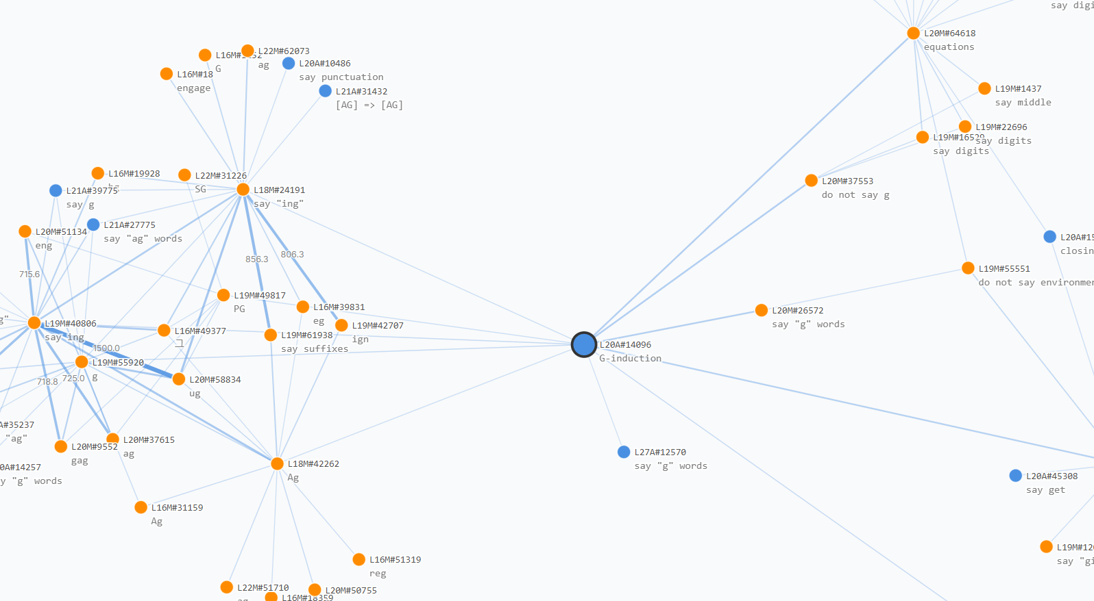
As an example, we start from a Lorsa feature at layer 20 that implements induction specific to g-related tokens (hover on top activations to see its z-pattern). The search process reveals a clear induction circuit: upstream features detect ending with g, ng, ag, and similar patterns, which feed into the induction head. Downstream, the circuit connects to features predicting g or G, as well as a number of confidence regulation features^[32] like suppressing g. The resulting global circuit is shown below.

The raw circuit produced by this search process can be quite information-dense and difficult to interpret. To make them more digestible, we apply a simple pruning strategy: we remove edges below a threshold strength and filter out standalone nodes. The interactive visualization below allows exploration of these pruned atlases with adjustable edge strength thresholds.

We provide several additional global circuits seeded from other features in the model (select seed feature in the dropdown menu). For instance, starting from an Annoyance feature, we find it activated by a number of feature clusters like 怒 (anger), 不屑 (scorn), holding grudges, and had enough.

These global circuits bring us closer to discovering the underlying connections that explain general model behavior. We hope to find more structural patterns such as motifs and other phenomena^[33] along this direction. However, several obstacles remain.

A primary challenge is the large number of possible connections. As model size grows, analyzing all features and connections becomes intractable in terms of both compute and memory. However, global connections to and from a feature are often sparse, as we observe in the global weights above:

Another concern is that our current global weight analysis often resembles feature clustering rather than discovering algorithmic-like end-to-end circuits. One explanation is that lorsa and plt features only connect to adjacent layers, making global weights short-range. An embedding-to-output path passes through up to 56 intermediate layers, requiring many search iterations to trace. This makes it difficult to see the broader algorithmic structure. A potential solution is to introduce cross-layer connections (see §?).

The global weight framework naturally extends to QK circuits, allowing us to compute expected attention patterns between query-side and key-side features. However, interpreting these QK global weights is challenging for similar reasons to the softmax problem in logit prediction (see §?): discriminative attention patterns are mixed with shared background scores. We plan to revisit QK circuit analysis after developing better approaches to isolate these components.

If we can improve global weight analysis, particularly efficiency, it may become possible to reason about model behavior from a broader perspective and explain failures on edge cases like adversarial examples^[2,34]. We plan to prioritize this direction in the near future.

Evaluation

In this section, we evaluate the effectiveness of the trained CRM and the attribution graphs derived from it. Following the evaluation framework proposed by Ameisen et al.^[8], we assess performance along three dimensions:

• Interpretability: We evaluate feature interpretability through automated scoring and assess the quality of the replacement layers by measuring reconstruction fidelity.
• Sufficiency: We quantify sufficiency using replacement score and completeness score as metrics to measure the proportion of error nodes in the circuit and the influence of these nodes on the final logits, thereby quantifying how well attribution graphs capture model behavior.
• Mechanistic Faithfulness: We perform matched perturbation experiments on both attribution graphs and the original model, measuring whether interventions on feature activations produce consistent downstream effects—i.e., whether the attribution graph accurately predicts the causal consequences of perturbations in the original model.

Prior to presenting our results, it is important to note that introducing Lorsas into the replacement model is a double-edged sword. While Lorsas enable understanding attention-mediated interactions, they also introduce additional approximation errors. The reconstruction fidelity of the CRM is thus additionally bounded, resulting in lower sufficiency metrics. This trade-off is quantified and discussed throughout the evaluation. As a result, we believe the addition of Lorsas fundamentally adds to the capability of the CRM despite newly introduced errors.

Replacement Layers Evaluation

We quantitatively assess the quality of the trained replacement layers by measuring normalized reconstruction error and explained variance. These metrics characterize how accurately the replacement layers approximate the computations of the original model components.

We also compare the reconstruction error of Lorsa and MHSA across sparsity levels. As a baseline, we control MHSA sparsity by applying AbsTopK to its concatenated \mathbf{z} vector, retaining the K channels with the largest absolute activations, analogous to the approach in §?. Lorsa achieves lower reconstruction error than MHSA even at twice the level of sparsity.

Attribution Graph Evaluation

Due to computational constraints, all experiments in this subsection are conducted with 8× expansion replacement models.

Computing Indirect Influence Matrix

Measuring the sufficiency and faithfulness of our replacement model depends on the indirect effect^[35,36,37], which describes the overall causal effect of an upstream node on a downstream node through all possible paths.

Indirect effect can be derived from the direct effect by iteratively aggregating paths of increasing lengths (mediated by more intermediate nodes). Starting from the attribution graph A \in \mathbb{R}^{N \times N} described in §?, where N is the number of nodes in the graph, and A_{ji} represents the direct contribution from node i to node j, we first preprocess it to get the normalized direct effect\hat{A}_{ji} = \frac{|A_{ji}|}{\sum_{k=1}^N |A_{jk}|},

where we rescale direct effect towards any target node to be all positive and sum up to 1. Indirect effect is then computed as:

Each term \hat{A}^k accumulates all k-hop paths, weighted by the product of edge weights along each path. The entry B_{ji} thus encodes all indirect influence that node i exerts on node j through paths of all lengths.

In practice, a complete attribution graph faithful to our replacement model still contains hundreds of thousands of nodes, making it intractable either to compute the complete attribution graph in adjacency matrix A or to compute the indirect influence matrix B from such a large A. We therefore adopt a greedy approximation to reduce the total node number: beginning from a subgraph containing only the logit nodes, we iteratively expand the subgraph by selecting, at each step, the node that maximizes influence on the current frontier. This procedure terminates once a predefined node budget is reached, yielding a compact subgraph that preserves the most influential pathways.

Sufficiency

In this subsection, we assess the sufficiency of the attribution graphs using two metrics proposed by Ameisen et al.^[8]: the graph replacement score, which captures how completely the graph traces information flow from embedding nodes to logits, and the graph completeness score, which quantifies the proportion of each node's indirect influence attributable to features rather than error nodes. A comparison of these scores between CRM and Transcoder-only replacement model illustrates how Lorsas affect the extent to which the attribution graphs suffice to explain model behavior.

For an attribution graph with \mathcal{N} nodes, we denote the sets of embedding nodes, feature nodes, and error nodes as \mathcal{E}, \mathcal{F}, and \mathcal{R}, respectively. The replacement score is defined as: S_{\text{r}} = \frac{\sum_{i \in \mathcal{E}} B_{\text{logit}, i}}{\sum_{i \in \mathcal{E} \cup \mathcal{R}} B_{\text{logit}, i}}.A higher replacement score indicates that the reconstruction error introduced by the graph has less actual impact on the output logits. The completeness score is defined as:S_{\text{c}} = \frac{\sum_{j \in \mathcal{N}} \left(1 - \sum_{i \in \mathcal{R}} \hat{A}_{ji}\right) B_{\text{logit}, j}}{\sum_{i \in \mathcal{N}} B_{\text{logit}, i}}.A higher completeness score indicates that, for the most influential feature nodes, a greater proportion of their indirect influence originate from features or embeddings rather than error nodes.

As expected, the CRM consistently yields a strictly lower replacement score than the Transcoder-only replacement model under the same node budget, since Lorsas introduce additional error nodes into the attribution graph, increasing the proportion of error-to-logit paths. Notably, however, we observe that this gap narrows: as the node budget and Top-K of CRM increase, the replacement score approaches that of the Transcoder-only replacement model, suggesting that the impact of these additional error nodes can be mitigated by training CRMs with larger dictionary sizes or lower sparsity.

Moreover, the CRM consistently achieves comparable or higher completeness scores than the Transcoder-only model under the same setting. We attribute this to Lorsas decomposing cross-token information flow into finer-grained paths, effectively replacing direct error-to-feature edges across tokens in Transcoder-only attribution graph with intermediate Lorsa feature nodes that better account for the sources of target feature node's indirect influence.

Mechanistic Faithfulness

Attribution graphs capture the internal mechanisms of the CRM, which, due to the reconstruction errors introduced by Transcoders and Lorsas, may deviate from the behavior of the underlying model. It is therefore essential to verify that the replacement model remains faithful to the original. Following Ameisen et al.^[8], we conduct three kinds of validation experiments to comprehensively assess whether both the replacement model and its derived attribution graphs faithfully reflect the underlying model's mechanisms.

Validating Indirect Influence within Attribution Graph

We first assess whether the influence metrics derived from the attribution graph accurately predict the causal impact of feature ablation on the underlying model's output. Specifically, for each ablated feature i, we measure the KL divergence between the original and ablated output logits as ground truth, and compute the Spearman correlation between the KL divergence values and the feature's direct influence \hat{A}_{\text{logits}, i} and indirect influence B_{\text{logits}, i}, using absolute feature activation as the baseline.

We construct attribution graphs from 100 prompts and, for each graph, individually ablate each active feature to compute the Spearman correlation. Indirect influence correlates most strongly with causal impact, followed by direct influence, with both substantially outperforming the feature activation. The correlation decreases slightly with larger Top-K, likely due to the inclusion of many low-influence features that introduce noise into the computation. As a result, it shows that "important" features indicated by our attribution graphs are highly consistent with those of the actual model behavior.

While the previous experiment validates influence at a global level from features to logits, we further examine at a finer granularity whether the indirect influence between individual feature pairs faithfully reflects the mechanisms of the underlying model.Using the same 100 prompts, we construct attribution graphs and identify the 512 features with the greatest influence on the logits in each graph. For each such feature, we ablate it and measure the resulting changes in activation of downstream features within 3 layers, computing the Pearson correlation between these changes and the corresponding indirect influence scores. We observe Pearson correlations of at least 0.62 in CRM across different sparsity settings, indicating that the graph faithfully captures the causal structure of the underlying model not only globally but also at the level of individual feature interactions.

Figures below show results from three randomly sampled examples, illustrating how well the pairwise feature influence predicts actual activation changes. Only a few points exhibit low predicted values but high actual values, confirming that the graph-based indirect influence reliably captures the actual effects between features.

Evaluating Faithfulness of CRM

To assess the overall mechanistic fidelity of the CRM, we introduce perturbations at an upstream layer and compare the resulting downstream effects in the underlying model with those propagated through the CRM. The degree of agreement between these two pathways indicates how faithfully the CRM captures the underlying model's internal mechanisms.

In these experiments, we freeze the error nodes in the replacement models, ensuring that both the CRM and the Transcoder-only replacement model match the underlying model's behavior exactly prior to perturbation. We consider three categories of perturbation vectors applied to the residual stream at a designated intervention layer:

• Encoder directions: For an active feature at the intervention layer, we add its encoder vector, scaled to increase the feature's activation by 0.1, to the residual stream.
• Random directions: As a control, we apply a random rotation to the scaled encoder vector above before adding it to the residual stream.
• Upstream features: We increase the activation of an active feature at an upstream layer by 0.1 and propagate through the replacement model to the intervention layer. The resulting change in the residual stream serves as the perturbation vector.

For each perturbation type, we run forward passes through both the underlying model and the replacement model, and at every layer beyond the intervention point, compute the perturbation effect — the difference between the perturbed and baseline residual streams. We then measure the cosine similarity and normalized MSE between the perturbation effects of the two models. For the encoder-direction and random-direction experiments, we sample 512 active features per layer; for the upstream-feature experiments, we sample 512 active features each from layer 1 and layer 14 as perturbation sources.

As shown in the bottom row, the CRM(K=64) maintains high cosine similarity across perturbation types and intervention layers. For encoder and random directions, fidelity decreases at higher layers, while for upstream features the trend is reversed, possibly reflecting shifts in the model's internal activation distribution across layers.

Overall, the CRM and the Transcoder-only replacement model exhibit comparable perturbation fidelity, indicating that the introduction of Lorsas does not significantly compromise mechanistic faithfulness. The CRM shows slightly lower fidelity near the intervention point, but this gap narrows at downstream layers, likely because downstream Lorsas can capture shifting attention patterns despite some reconstruction error, while the Transcoder-only replacement model relies on frozen attention patterns.

Related Work

Sparse Dictionary Learning

Interpretable units are the fundamental building blocks of mechanistic interpretability and circuit tracing. Sparse Dictionary Learning has emerged as a principled approach for decomposing neural network activations into sparse features, with interpretability superior to natural units like neurons and attention heads.

Despite its distant origin^[38], sparse dictionary learning has recently gained momentum through the establishment of Superposition Hypothesis^[2,39,1], which suggests that a neural network represents more features than it has neurons. Building on this hypothesis, Sparse Autoencoders (SAEs)^[3,4] have been developed to disentangle sparse features from the natural superposition in the neural network activations. Methodological improvements on SAEs have been continuously made to tackle the unique challenges in sparse training ^{[12,13,14,40]}. SAEs have also proven their ability to extract features from various internal locations^[41,42,43], from different model architectures^[44,45] and from frontier models^[12,46]. Still, outstanding limitations and challenges remain in the performance and soundness of SAE-based feature extraction^{[47,48,49,50,51]}.

One restriction of SAEs is that they learn features from a transient, isolated point of the model, making it difficult to study the interaction between features and ensure faithfulness. Several architectural variants have been proposed to address this limitation. Transcoders^[6,7] employ an architecture identical to SAEs, but learn to predict MLP layer outputs from their inputs, bridging over the non-linearity in MLPs. Similarly, Lorsa^[9] sparsifies MHSA to disentangle attention superposition, allowing sparse feature connections passing through attention layer. Crosscoders^[52,53,54] employ multiple parallel encoders and decoders and a unified feature space to resolve superposition among different activation spaces, either cross-layer^[52] or cross-model^{[52,53,54,55]}. Cross-layer Transcoders (CLTs)^[8] follow an architecture similar to weakly causal crosscoders, but further decouple input and output spaces, allowing for simultaneous sparsification of all MLP computations while tackling cross-layer superposition.

Circuit Discovery

Circuit Discovery methods aim to uncover the causal dependencies between components of the model. Following the definition of Olah et al. (2020)^[56], a circuit is a subgraph of the model's full computation graph (a directed acyclic graph) that partially represents the model's computation under certain tasks. Nodes of the graph represent model components (e.g. neurons, attention heads, etc.) and edges mediate the influence between them. Recent advances in circuit discovery can be roughly categorized into two categories: improvements on proper elements serving as nodes (circuit units) and improvements on how to find the nodes and edges (tracing methodology).

Improvements on Circuit Units

Circuit units are the fundamental building blocks of circuit discovery. Whether the units are understandable for humans is crucial for whether the whole circuits are interpretable. Early circuit discovery methods (often referred to as variants of attribution or information flow, since they do not provide explicit graph structure) primarily focused on natural units of the neural network. Researchers have attempted to highlight relevant parts of the input (typically image) in CNNs using saliency maps before mechanistic interpretability was developed^{[57,58,59,60,61,62,63]}, where the units are directly pixels or regions in the input images. Methodologies then advanced to intermediate model components, including neurons^{[64,23,65,66]} and attention heads^[25,27,67], until recently when sparse dictionary learning methods have prevailed and sparse features become the dominant units for circuit discovery^[10,37,6,68]. Transcoder features and CLT features soon followed to enable inherent perception of model computation and allow for more robust and input-invariant circuit discovery^[7,6,8].

Improvements on Tracing Methodology

Another important direction of circuit discovery concerns how to trace important nodes and compute faithful dependencies between them. Most of the existing approaches fall into either of the following two groups: intervention-based or attribution-based.

Intervention-based methods intervene on the model, typically by changing the input or intermediate activations, and observe the downstream effects. Activation Patching (a.k.a. causal tracing, causal mediation) is the prevalent paradigm^[36], which runs the model on input A, replaces (patches) an activation with that same activation on input B, and sees how much that shifts the answer from A to B. This paradigm has been widely applied in interpretability studies^{[69,70,71,72]}. Meng et al. (2022)^[73] uses similar strategy to locate factual associations, and extends it to also edit the internal information to fix mistakes. Wang et al. (2023)^[27] develops Path Patching, which enables path-based intervention and applies it to the Indirect Object Identification task. Conmy et al. (2023)^[74] automates activation patching with a recursive patching procedure.

Attribution-based methods use attribution scores to guide the tracing process, which are first-order Taylor expansion terms. Unlike intervention-based methods, attribution-based methods do not require separate forward passes for each interested component, but only a backward pass to obtain all the gradients.

Early interpretability studies on CNNs use saliency maps, whose form is identical to attribution scores. Inspired by patching methods, Nanda (2023)^[75] introduces Attribution Patching, which still focuses on patching from a clean run to a corrupted run, but uses attribution scores to find important components, with a total of 2 forward passes and 1 backward pass. Syed et al. (2024)^[76] finds its performance is superior to automated activation patching methods. Several works follow this paradigm to improve the gradient approximation^{[77,78,79,80]}. Marks et al. (2025)^[37] extends attribution patching to SAE features and uses integrated gradients for better approximation. Ge et al. (2024)^[6] employs transcoders and separates OV and QK circuits to keep the computational graph linear. Kamath et al. (2025)^[30] follows up to trace attentional computation in a more systematic way by checkpointing attention paths. Ameisen et al. (2025)^[8] proposes CLT based attribution graphs for a complete understanding of the model's computation for a single prompt. It is worth noting that when studying linear effects^[6,8], the attribution scores are identical to simple input decompositions (i.e. W x = \sum_i W x_i)

Discussion

Alternative Approaches to Complete Replacement Models

Both CRMs and the checkpointing approach from Kamath et al.^[30] address the same challenge: exponentially growing attention-mediated paths between features. Both introduce sparse dictionary learning to add interpretable features to the attribution graph. However, their architectural choices lead to different trade-offs.

Kamath et al. checkpoint attention-mediated paths by training SAEs in the residual stream at each layer and computing gradient attributions between adjacent-layer features. This limits attribution edges to attention paths of length 1. However, this makes the attribution graph non-linear: the computational graph depends on the specific input. Additionally, checkpointing with residual stream SAEs cannot address §? because heads in the underlying model cannot be independently understood.

CRMs replace attention layers directly with Lorsa modules. All computational paths start from a source node, pass through the residual stream (where only layernorm and Lorsa attention patterns are applied), and end at a target node. This maintains a conditionally linear computation graph while directly addressing attention superposition. Each Lorsa feature has independently interpretable QK and OV circuits.

Dimensionality Collapse in Attention Outputs

Attention outputs exhibit strong low-rank structure: approximately 60% of directions account for 99% of variance^[81]. This dimensionality collapse is fundamental to the reconstruction quality and interpretability of attention SAEs and Lorsa layers.

Without initialization strategies that align feature directions with the active subspace of activations, attention replacement layers suffer from high rates of dead features and poor reconstruction. Weak attention replacement layers fail to capture the underlying attention mechanisms, preventing effective circuit tracing.

We conjecture that attention replacement models that ignore this structure accumulate reconstruction error in the residual stream across layers. This leads to attributions dominated by error nodes rather than interpretable features. Kamath et al.^[30] observe similar error accumulation in their attention replacement models, though they do not explicitly discuss dimensionality collapse or initialization strategies.

Lorsa Feature Families

Throughout the §?, we observed related Lorsa features sharing the same QK weight matrix. These feature families implement the same attention pattern but write different information to the residual stream. For example, in the §? case, features like Starts with, Say second, and End with all share QK weights but have distinct OV circuits for copying different character positions. Similar groupings appear in the induction and multiple choice examples.

This weight sharing reflects a fundamental architectural choice in Lorsa: QK circuits remain full-rank while OV circuits are reduced to rank-1. Experiments in the original Lorsa paper showed that reducing QK dimension significantly degrades performance. One reason is that rotary position embeddings were trained with a specific head dimension. Reducing QK dimension disrupts these position-dependent transformations, causing the replacement model to lose track of token positions.

More fundamentally, QK patterns represent high-level computation. The attention pattern depends on groups of features that collectively describe a functionality, not on individual feature semantics. In the string indexing example, all four features need to locate index-related positions regardless of which specific character they copy. This makes QK circuits natural candidates for weight sharing: multiple features reuse the same attention mechanism while specializing their output through distinct OV circuits.

In contrast, OV circuits behave like transcoders, performing feature-specific transformations from the key-side residual stream to query-side contributions. These transformations naturally decompose to rank-1 operations where each Lorsa feature reads specific input features and writes to specific output directions. The semantic specificity of OV circuits makes them unsuitable for sharing, while their rank-1 structure keeps the parameter count tractable even with thousands of features per layer.

Architectural Compatibility

The architectural compatibility we maintain for Lorsa layers enables CRMs to adapt to any modern transformer architecture. Most improvements to multi-head self-attention can be directly incorporated into Lorsa, preserving architectural choices such as causal masking, attention scaling, rotary embeddings, grouped query attention, and QK-layernorm. As transformer architectures evolve, our replacement methodology can incorporate these advances without fundamental redesign.

One open question is GLU-based MLPs. We do not use a gate mechanism for transcoders in this work, though gates might better capture the bilinear nature of modern GLU MLPs. However, gates introduce non-linearity that could complicate attribution tracing. To maintain linear attribution graphs, we could detach gradients for gate activations, treating them as constants during attribution computation. We leave this investigation for future work.

"Uninterested" Circuits

Attribution graphs sometimes fail to capture the mechanistic stories we care about. The core problem stems from softmax: when interpreting why a model chooses a particular token, we care about why that logit stands out among candidates, not just its absolute value. However, standard attribution tracing tracks absolute contributions to the target logit, making it difficult to distinguish discriminative signal from shared background.

We observed this in the §?. When the model predicts the last character of "Craig" versus "Frank" in confounding contexts, the logit difference between "g" and "k" accounts for only around 30% of the total logit magnitude (logits: g = 36.0, k = 26.2 for "Craig"; g = 27.0, k = 43.0 for "Frank"). The remaining 70% comes from features that boost all plausible character predictions uniformly. Attribution graphs dominated by these shared features obscure the discriminative circuits.

Two potential approaches might help isolate discriminative features for logit prediction. First, we could trace from the target logit vector projected onto the nullspace of a manually designed general feature subspace. This removes shared contributions that apply across all candidate tokens. Second, we could perform graph diffing by computing attribution graphs for both the target token and a confounding alternative, then eliminating shared features and circuits. Both methods require manual design choices about what constitutes "uninteresting" background versus discriminative signal.

These approaches become more complex for QK tracing, where softmax operates on attention scores rather than output logits. RoPE (rotary position embeddings) further complicates the picture: it applies position-dependent transformations to queries and keys, making it difficult to cleanly eliminate bias-bias feature interactions through QK circuits. In RoPE models, bias-bias interactions often implement position-related QK circuits that we cannot simply factor out. Addressing the softmax comparison problem in attention mechanisms likely requires deeper investigation beyond current attribution methods.

Inactive Features and Inhibitory Circuits

A related challenge is understanding inhibitory circuits where features actively suppress other features. Anthropic's recent work on attribution graphs discusses this extensively under "The Role of Inactive Features & Inhibitory Circuits", showing how the absence of expected features can be just as mechanistically important as their presence. CRMs do not directly solve this problem, as attribution graphs still primarily surface active features.

However, global weights offer a potential path forward. When a feature we expect to activate remains inactive, we can inspect its typical upstream contributors via global weights to understand what normally causes it to fire. These global weights capture the average connectivity patterns across many prompts, revealing which features consistently excite or inhibit the target. If the typical positive contributors are also inactive, we recursively trace further upstream through their own global weight connections until we find where the expected activation pathway diverges from its typical pattern. This backward search reveals which early features failed to activate, breaking the chain that would normally lead to our target feature.

Conversely, if the typical upstream contributors are active as expected, we can search for strong negative global weights pointing to the target feature. These inhibitory connections reveal features that actively suppress the target when present. By examining which of these inhibitory features are active on the current prompt, we can identify the specific suppression mechanism at work. This approach essentially uses global weights as a reference template, allowing us to diagnose deviations from normal activation patterns by comparing what typically happens against what actually occurred on a specific input.

Unexplained Phenomena

The attribution challenges discussed above limit our ability to fully explain certain circuits. When discriminative features are obscured by shared background contributions, or when critical features remain inactive due to inhibition, the resulting attribution graphs may miss key computational pathways. Additionally, reconstruction error can accumulate across layers, creating noise that further obscures the mechanistic story. These limitations manifest in several unexplained phenomena from the §?.

In the acronym example, after the model identifies "Analytics" and produces "A" for the first letter, why doesn't it continue by attending back to "Analytics" to output "n" for the second letter? Instead, the model appears to encode all necessary letter information in parallel during early processing, but the mechanism by which it selects which letter to output at each position remains unclear.

The §? examples raise questions about variable binding. When the model sees a="Craig" followed by assert a[0]==', how does it bind the variable name "a" to the string "Craig" and maintain this binding across multiple tokens? The attribution graphs show features that recognize variable names and string literals, but the binding mechanism itself—how the model associates "a" with its value rather than other variables in context—does not surface clearly in the feature-level circuits we observe.

In the §? case, we identified features that distinguish correct from incorrect answer options, but the deeper question remains: how are these features computed? The model must somehow evaluate factual knowledge (e.g., when World War II ended) and compare it against each option's content. While we observe the final discrimination in option-specific features, the computational pathway that encodes and retrieves the relevant factual knowledge before this discrimination occurs is not captured in our graphs. This suggests either that the crucial computation happens in ways our current attribution methods cannot surface, or that important features remain unidentified in our current replacement models.

Open Source Replacement Models

Training replacement models at scale requires substantial computational resources and engineering effort, which suggests the need for open-source replacement models to facilitate reproducibility and collaboration.

The mechanistic interpretability community has made significant progress in openly releasing trained sparse dictionaries. Our team previously released Llama Scope^[41], extracting millions of SAE and transcoder features from Llama-3.1-8B. Google DeepMind released GemmaScope^[42], training SAEs and transcoders across multiple Gemma 2 model sizes and layers. More recently, GemmaScope 2^[43] extended this work with cross-layer transcoders (CLTs) and per-layer transcoders (PLTs), placing greater emphasis on circuit tracing capabilities.

We plan to release Llama Scope 2, focusing specifically on complete replacement models for circuit tracing. Our initial release will include open-source Lorsas and transcoders trained on Qwen3-1.7B with the configurations presented in this work, with more models supported in the future. All models and resources will be publicly available at OpenMOSS-Team/Llama-Scope-2. A production-ready version of our training and analyzing codebase, with documentation and tutorials, is currently being finalized and will be released alongside.

Cross Layer Replacement Models

Cross-layer transcoders^[8] have demonstrated that features can exist in superposition across multiple MLP layers. We suspect that this cross-layer superposition also occurs in attention layers and between different layer types. Features may be jointly represented across both attention outputs and MLP outputs. If this hypothesis holds, it would be beneficial to design replacement models where both Lorsa and transcoder features can write to all downstream attention and MLP outputs, creating a unified feature space that resolves superposition across computational blocks.

However, unrestricted cross-layer connections introduce a quadratic explosion in the number of possible feature interactions. For a model with L layers and F features per layer, allowing arbitrary cross-layer connections yields O(L^2 F) potential edges, making both training and analysis computationally intractable. A more practical approach is to limit cross-layer connections to a fixed window of adjacent layers (we might call these short-range or windowed cross-layer connections). This design choice is motivated by the observation that most cross-layer superposition appears concentrated in nearby layers rather than spanning the entire residual stream. By restricting each feature to write only to the next few layers, we can balance the benefits of resolving cross-layer superposition with computational efficiency.

Exploring these architectural variants remains an important direction for future work. The right balance between expressiveness and scalability will depend on empirical measurements of how far cross-layer features typically extend and whether the added complexity improves circuit tracing quality.