Introduction

Understanding the underlying mechanisms of large language models is critical to mechanistic interpretability research. One of the main challenges is that most neurons and attention heads cannot be independently understood. The field has identified this problem as superposition^[1,2]. This hypothesis suggests that there might exist true features that the model is using to represent information, but these features are often smeared across multiple neurons or attention heads. An active direction in addressing this problem is 1) to find these true features and 2) understand how they interact with each other via model parameters (i.e. circuits).

Sparse dictionary learning methods, particularly sparse autoencoders (SAEs)^[3,4], have emerged as a promising approach to extract monosemantic features from language models. A variant called transcoders^[5,6,7] makes circuit identification easier by approximating MLP outputs with sparse features. Recent work has used transcoders to build attribution graphs (visual representations of how features influence model outputs) for specific prompts^[6,8].

However, these approaches share a critical limitation: §?. Existing methods decompose MLP computation but treat attention patterns as given, leaving attention superposition unresolved. We address this by introducing complete replacement models (CRMs), which combine transcoders for MLPs with Low-Rank Sparse Attention (Lorsa)^[9] modules for attention layers. This gives us interpretable features for every computational block.

Complete replacement models. In §?, we introduce CRMs, which replace each attention and MLP layer with a sparse replacement layer trained to approximate the original layer's output. Each Lorsa feature has its own QK circuit (determining where to attend) and rank-1 OV circuit (determining what to read and write), making attention computation fully decomposable. By freezing attention patterns and layernorm denominators during attribution, we convert the model into a linear computation graph where all feature interactions flow through interpretable virtual weights. This architectural completeness is key to both efficient attribution and global weight analysis.

Why attention matters. Training SAEs on attention outputs can extract monosemantic features^[10,11], but these features may still be collectively computed by multiple heads. This makes it difficult to trace how attention patterns form, a process called §?. Lorsa solves this by decomposing attention into sparse, independently interpretable features, each with its own QK and OV circuits.

Complete attribution graphs. In §?, we show how CRMs convert all attention-mediated paths into combinations of interpretable feature interactions. This eliminates the exponential growth of possible paths between features and enables complete attribution graphs that trace both MLP and attention circuits.

Revisiting the biology of language models. In §?, we apply CRMs to study how Qwen3-1.7B implements specific behaviors. In string indexing tasks, we trace how the model selectively retrieves characters at different positions through shared attention feature families. For induction, we identify distinct subcircuits operating at different depths: lower layers perform relation-keyed binding while higher layers execute generic retrieval. These case studies reveal attention-mediated feature interactions that were previously hidden in transcoder-only analyses.

Global circuits. In §?, we show how architectural completeness unlocks efficient global weight analysis. Because all feature interactions flow through static virtual weights rather than input-dependent attention patterns, we can compute expected attributions over distributions and construct global circuit atlases. These reveal canonical computational patterns such as induction circuits at the feature level for the first time.

Evaluation. In §?, we train CRMs for Qwen3-1.7B and evaluate them across three dimensions: interpretability (feature quality and reconstruction fidelity), sufficiency (how well attribution graphs capture model behavior), and mechanistic faithfulness (whether interventions match predictions). While Lorsa introduces additional reconstruction error, the resulting attribution graphs achieve comparable faithfulness to transcoder-only models while providing complete circuit coverage.

Replacement Layers

Replacement layers are sparse, interpretable modules trained to approximate the computation of individual attention or MLP modules in the underlying model. Each replacement layer learns a dictionary of features and uses sparse coding to reconstruct the original layer's output: sparse codes are computed from the layer inputs, then decoded through the dictionary to approximate the original output. Conceptually, the original layer is "sandwiched" between the encoder (which computes sparse features from inputs) and the decoder (which reconstructs outputs from these features), allowing us to decompose the computation into interpretable, monosemantic components. By combining replacement layers for all underlying layers, we obtain a §? that rewrites the model's computation in a more interpretable form.

Transcoders

Transcoders^[6,7,8] are replacement layers that approximate the computation of an MLP layer. In this work, we use the per-layer version instead of cross-layer transcoders^[8] for both conceptual and engineering simplicity. A Per-layer Transcoder (PLT) has the same architecture as Sparse Autoencoders (SAEs) ^[3,4], but learns to approximate downstream activations instead of its original input.

Concretely, given an MLP input activation, denoted as \mathbf{x} \in \mathbb{R}^d, the transcoder computes the feature activation as:

where \mathbf{W}_\text{enc} \in \mathbb{R}^{F \times d} is the encoder weight matrix. The input is encoded into a feature activation space with F \gg d dimensions, followed by a Top-K sparsity constraint to select the K strongest features and set others to zero^[12]. Alternative sparsity constraints such as BatchTopK^[13] and JumpReLU^[14] should have similar effect^[15].

The sparse feature activations are then decoded to the output space as:

where \mathbf{W}_\text{dec} \in \mathbb{R}^{d \times F} is the decoder weight matrix, and \mathbf{b}_\text{dec} \in \mathbb{R}^d is the decoder bias.

The transcoder is trained to simply minimize the mean squared error between the decoded output and the original output \mathbf{y} \in \mathbb{R}^d:

Low-Rank Sparse Attention (Lorsa)

Lorsa^[9] is designed as a sparse replacement model for attention layers. As the attention counterpart of transcoders, it is also trained to find a sparse representation of the attention layer output, while also accounting for how these sparse features are computed from attention input.

Attentional Features and Attention Superposition

These two terms were first introduced in Jermyn et al. (2023)^[16] and Jermyn et al. (2024)^[17]. We further extended investigation of this topic in our paper Towards Understanding the Nature of Attention with Low-Rank Sparse Decomposition^[9]. These works assumed and provided evidence that we can extract monosemantic attentional features from superposition in the attention layer.

Our current understanding on attentional features is that they each has:

• A QK circuit reflecting how they choose to attend from one token to others;
• A rank-1 OV circuit reading a specific set of features from key-side residual streams and writing to the query side.
• Overcompleteness and Sparsity: The underlying attention layer learned to represent orders of magnitude more attentional features than it has heads, if and only if they are sparsely activated at any given position. This is analogous to the definition of superposition in activation spaces^[2].

Following the definition of attentional features, we design Lorsa to have an overcomplete set of sparsely activating attention heads, each of which has a rank-1 OV circuit and a QK circuit with the same dimension as the underlying attention layer. In practice, we adopt weight sharing across groups of heads(TODO: Add a section ref) to maintain scalability. But for conceptual simplicity, we illustrate the architecture with independent QK circuits.

Lorsa QK Circuits

Let \mathbf{X}\in \mathbb{R}^{l \times d} denote the input of the attention layer, where l is the sequence length and d is the dimension of the input. The QK circuit of a Lorsa head with head dimension d_h is computed as follows (we omit head index for simplicity):\mathbf{Q} = \mathbf{X} \mathbf{W}_Q; \mathbf{K} = \mathbf{X} \mathbf{W}_K,where \mathbf{W}_Q, \mathbf{W}_K \in \mathbb{R}^{d \times d_h} are the QK weight matrices. Attention pattern is then computed as:\mathbf{P} = \text{softmax}(\mathbf{Q} \mathbf{K}^T),where \mathbf{P} \in \mathbb{R}^{l \times l} is the attention pattern. Lorsa QK circuit is architecturally equivalent to the underlying attention layer.

Since attention architecture of the underlying model varies across models, we adopt an §? to apply causal mask, attention scale^[18], rotary embedding^[19], grouped query attention^[20] and QK-layernorm^[21,22].

Lorsa OV Circuits

The OV circuit of a Lorsa head is computed as:\textbf{v} = \mathbf{X} \mathbf{w}_V; \textbf{z} = \mathbf{P} \textbf{v},where \mathbf{w}_V \in \mathbb{R}^{d} is the value weight projection. This maps the input to \mathbf{v}, which is a scalar at each position. Then the attention pattern moves these values to the query side as feature activation \textbf{z} \in \mathbb{R}^l at each position. Similar to transcoders, we apply a Top-K sparsity constraint (along the head dimension) to select the K strongest features and set others to zero^[12]. For each position, we have a set of selected features denoted as \mathbf{S}_c, c=1,2,\cdots,l.

The output of this head at a given position c is simply:\textbf{y}_c^\prime = \sum_{s\in\mathbf{S}_c} \textbf{z}_s \mathbf{w}_{O,s},where \mathbf{w}_{O,s} \in \mathbb{R}^d is the output weight of feature s. Training a Lorsa layer is similarly minimizing the MSE loss between Lorsa output \mathbf{y}_c^\prime and attention output \mathbf{y}_c at each position.

Visualizing Features

Our understanding of sparse features are based on their mathematical and statistical properties, typically shown by their direct logit attribution (DLA) and their top activation contexts. Below we show an example Transcoder feature from layer 18 of Qwen3-1.7B, which activates on tokens starting with "g" or similar patterns in the latinization of other languages:

Lorsa features can be inspected in similar way. In the visualization of Lorsa features, we further provide the z-pattern, which can be observed by hovering activated tokens. Below is an example Lorsa feature at layer 22 of Qwen3-1.7B, which attends to "g" tokens and predicting next tokens to end with "g":

Training Setup

We train replacement layers on Qwen3-1.7B with varying capacity settings, exploringK \in \{64, 128, 256\} combined with feature activation space dimensions of 16,384 and 65,536. Detailed training configurations are provided in the appendices:Dataset, Learning Rate, and Initialization.

From Transcoder-Only to Complete Replacement Models

In this section, we start from a specific attribution graph obtained by a transcoder-only replacement model, and show four fundamental problems of it. Then we introduce how a complete replacement model (i.e. a model with both transcoder and lorsa replacement layers) can solve these problems.

Transcoder-Only Replacement Models

The idea of building attribution graphs with MLP replacement layers was first proposed in our previous work Automatically Identifying Local and Global Circuits with Linear Computation Graphs^[6], but not investigated deep enough.

Using transcoders for direct feature-feature interactions computed by MLP blocks, with attention modules left as is. By "freezing" attention patterns and layernorm denominators, the computation of the underlying model can be described as a linear computation graph given a specific input^[23]. This makes attribution We can further prune the graph to isolate a subgraph of interest for easier digestion.

This methodology was greatly improved by Ameisen et al.^[8] in many aspects including attribution and pruning algorithm, visualization interface, evaluation and global weight analysis. Importantly, they proposed to replace all MLP modules with a Cross-Layer Transcoder (CLT) rather than a set of Per-Layer Transcoders (PLTs) to combine features that might exist across multiple MLP layers^[24] for simpler attribution graphs.

The Problem of Missing Attention Circuits

This attribution gives us a partial picture of the underlying model behavior. However, it fails to explain which attention head(s) is responsible for edges between two features from difference positions. Concretely, this breaks down to four fundamental problems:

1. §?: Despite a bunch of existing work on identifyng independently interpretable attention heads^{[25,26,27,28]}, most heads in a transformer language model cannot be independently understood^[29].
2. Exponential Growth of Attention-Mediated Paths: Consider two transcoder features separated by P tokens and L layers. The edge connecting these two features has \sum_{k=1}^{L} \binom{L}{k} \binom{P+k-1}{k-1} possible paths (under the assumption that each layer has only one attention head).
3. Head Loading^[30] in One Attention Layer: Even in cases where a single path almost exclusively contributes to an edge, we still need to quantify the amount that each attention head is responsible for mediating its corresponding attention layer.
4. Attention-Mediated Interaction in one Residual Stream: Since attention layers can attend from one token to itself, attribution inside a residual stream should also take into account the attention-mediated interaction. We show how this affects global weight analysis in §?.

Complete (Local) Replacement Models

With Lorsas, we now have a sparse replacement layer for each original computational block. Combining these replacement layers yields a Complete Replacement Model (CRM), which adopts a distinct yet related parameter set to the underlying model. The CRM and underlying model share the same overall architecture, but the CRM's neurons (i.e., transcoder features) and attention heads (i.e., lorsa heads) show substantially greater monosemanticity.

The forward pass of any prompt is taken over by the CRM and computes as follows:

1. Tokens pass through the same embedding layer, which is by itself an interpretable transformation of the input tokens.
2. Upon reaching an attention layer, we use its corresponding Lorsa module to compute its output at each token position. The same applies to transcoders for MLP layers.
3. Lorsa attention patterns and layernorm denominators are freezed after they are computed. This means we treat them as a constant in the replacement model, instead of being computed from their inputs.
4. Following Marks et al. and Ameisen et al., we add an error term to the output of each replacement layer's output to exactly make up the reconstruction error so that later layers will receive the same input as the original model.
5. Finally, we unembed the output to get the same final logits as the original model.

Compared to a transcoder-only replacement model, a complete replacement model offers us a more complete picture of the underlying model behavior. It also has many good properties for attribution, which we will discuss later on. However, these come at a cost of additional error terms from Lorsas. We will measure the impact of these error terms on attribution in TODO:SectionRef.

Including attention replacement layers in a replacement model makes it complete in the sense that it is designed to attack superposition happening in both attention and MLP layers. However, it is still local because of 1) frozen lorsa attention patterns and layernorm denominators 2) and uninterpretable error terms. Both are dependent on specific model inputs but we choose not to explain them in this phase. We will later show how we further explain lorsa attention patterns in TODO:SectionRef.

Building Complete Attribution Graphs

The algorithm we use for attribution is generally similar to that in transcoder-only models^[6,7,8]. That is, for any two nodes in a local replacement model, the attribution between an upstream (source) node and a downstream (target) node is defined as A_{s\rightarrow t} := a_s w_{s\rightarrow t} where a_s is the activation of the source node, and w_{s\rightarrow t} is the sum over all possible paths from the source to the target.

A good property in CRMs is that direct interaction between any two nodes is mediated by no more than one paths. So the term "edge" in graph contexts and "path" in Transformer contexts are equivalent. We will be using these terms interchangeably in the rest of this work.

Since the residual stream mediates all inter-node interactions, attribution between any two nodes depends only on how the source node writes to the residual stream and how the target node reads from the residual stream. We abstract generic encoder and decoder vectors to unify the measuring of these read/write abilities of all node kinds. The generic encoder vector \mathbf{w}_{\text{enc}, t} is given by

Similarly, the generic decoder vector \mathbf{w}_{\text{dec}, s} for a source node s is given by

Consider any source node s from position i and a target node t at position j s.t. i\le j, the graph weight is given byA_{s\rightarrow t} = a_s P_{i,j}^t \mathbf{w}_{\text{dec}, s}^\top \mathbf{w}_{\text{enc}, t} = a_s P_{i,j}^t \Omega_{s\rightarrow t},where P_{i,j}^t is the attention pattern between positions i and j computed by the target node t. Transcoder features and logits do not have attention pattern, in which case we set an identity attention pattern P^t = I without losing generality. \Omega_{s\rightarrow t} := \mathbf{w}_{\text{dec}, s}^\top \mathbf{w}_{\text{enc}, t} is defined as the residual-direct virtual weight^[23] between two features.

For a given prompt, we first run a forward pass to get all necessary node activations and Lorsa attention patterns. Then we can compute the connections between nodes with source node activations, attention patterns and virtual weights. This will give us a complete linear attribution graph for the given prompt.

In practice, we still apply a gradient-based implementation^[6,8] on CRMs to compute the attribution by stopping gradient propagation at the Lorsa attention patterns and layernorm denominators, where the computation is equivalent to the forward perspective we introduced above. The main reason to do this is efficiency and backward compatibility.

We refer readers to TODO:SectionRef for how we prune the attribution graph for easier comprehension.

An Example Complete Attribution Graph

After pruning and human distillation, we can describe mechanistic hypotheses about the model's behavior for any given prompt. We study a similar prompt to Ameisen et al. for more straightforward comparison. The model takes "The National Digital Analytics Group (ND" as input and is able to complete the acronym by predicting "AG" as the next token.

The overall structure of the attribution graph is similar to the established conclusions from transcoder-only models: The model learns a group of "First Letter" features at early layers of the model (e.g., A-initial and G-initial features in the graph above). A group of "First Letter Mover" features then moves them to the last token position to enhance probability of token "AG" being predicted.

Compared to transcoder-only models, a complete attribution graph identifies important attention heads responsible for the model's behavior (moving first letters in this example). We can then learn from this graph that the Say A Lorsa features are reading a set of A-initial features from "Analytics" position and writing to the residual stream to encourage "Saying A". This is the OV perspective of describing an attentional feature.

We also want to understand why this features attend to the specific residual stream position. By looking at features contributing to the attention pattern between the last token and "Analytics" position, we can see that the query side (last token) has a set of Acronyms Unfinished features searching for the next words in the acronym. The key side ("Analytics") has a group of middle of titles features indicating that this word is likely to be a middle word of a title. Similarily, the Say G-ending Lorsa attention pattern is mainly contributed by a group of end of titles features on the key side and Acronyms Unfinished features on the query side. We call this process QK tracing.

QK Tracing

The idea of QK tracing in the context of sparse feature circuits was first introduced in He et al.^[10], and further illustrated in more detail in Kamath et al.^[30]. We can leverage the bilinear nature of attention score computation. Since attention scores are computed as dot products between query and key vectors—which are linear transformations of the residual stream—we can decompose each attention score into a sum of interpretable terms.

Specifically, by expanding the residual stream at query and key positions as sums of feature activations, bias terms, and residual errors, the bilinear form naturally decomposes into feature-feature interactions (inner products between query-side and key-side features), bias interactions, and error terms. This allows us to explain why an attention head attends to particular positions in terms of which features on the query side interact with which features on the key side. For a detailed mathematical treatment, we refer readers to Kamath et al..

However, attention scores are normalized by softmax to form a probability distribution, which means we cannot simply examine how attention scores form at one position in isolation. Suppressing other positions will affect the attention pattern at the target position. This same issue arises in logit attribution as well. We refer readers to §? for further discussions.

Navigating an Attribution Graph

Now we demonstrate how we visualize and navaigate an attribution graph to form mechanistic hypotheses for the example above. The interactive visualization below shows a heavily pruned attribution graph. Nodes in the graph represent active features at different tokens and different layers with influence strength above a certain threshold. These include token embeddings, predicted logits, Transcoder features and Lorsa features. Error nodes are for uncaptured residuals in either Transcoders or Lorsas.

You can click on any node to inspect the detailed information of the feature, along with its incoming and outgoing connections to any other nodes. By navigating through the primary connections, we can trace how Lorsa OV and transcoder paths influence the model's behavior.

For any Lorsa feature, we can click on it and select the "QK Tracing" tab to see the top marginal and pairwise feature contributions to the attention scores between the target (query) position and the position with largest z-pattern contribution. These nodes are not displayed in the graph, but we can click on them in the QK tracing tab to see their detailed information.

Causal Validation: Reversing Word Order

Feature steering offers a way to verify that the mechanisms captured by the attribution graph are causally real: if manipulating features produces changes consistent with the graph's predictions, the identified mechanism is likely genuine. The graph above suggests that the model's prediction of "AG" relies on "middle of titles" features activating on "Analytics" and "end of titles" features activating on "Group." To test this, we can swap the activation positions of these features and expect the model to output "GA" instead of "AG," reflecting the reversed positional signals.

Specifically, we swap the activations of the "middle of titles" and "end of titles" features between the "Analytics" and "Group" positions. To prevent downstream self-correction by the model, we further scale up the swapped activations — amplifying the "end of titles" features at "Analytics" and the "middle of titles" features at "Group" by multiplicative factors.

Lessons Learned from Attribution Graphs

Investigating attribution graphs reveals

Revisiting the Biology of Language Models

In this section, we will present several behaviorial case studies to see what we can learn about the biology of the underlying model with the complete replacement model. We are interested in cases where the model's behavior is better revealed by the complete replacement model.

Specifically, we will mainly showcase 3 types of attention head interactions:

• Q-composition: upstream attention features compose with downstream attention features as the query side of the attention pattern;
• K-composition: upstream attention features as the key side of the attention pattern;
• V-composition: upstream attention features as the value of the downstream attention features.

String Indexing

We start with a Python code completion example where the model takes

a="Craig"
assert a[0]==

as input. The model is able to complete the assertion by predicting "C" as the next token, i.e. the first character of the string stored in variable a.

The attribution graph reveals how the model performs string indexing: early layers detect extract the first letter of the string through a group of C-Initial features. Simultaneously, the model recognizes that the token "0" represents a First element index.

In the last token position, the Starts with Lorsa features aggregates information from the "0" position to inform downstream heads to retrieve the first character of the string. The Say C Lorsa feature then reads from the "Craig" position and copies its first letter to the last token residual stream to encourage predicting "C".

A similar structure is observed for a[1]. The model recognizes "1" as representing a The second position, and early layers detect the second letter of Craig through Second letter is r features. The Say second Lorsa feature aggregates information from the index position, informing the Say r Lorsa feature to retrieve the second letter.

For a[-1], the model recognizes "-1" as an Last position and activates the End with features to retrieve the last character from "Craig".

Discussion and Open Questions

Shared Prefix. It is worth noting that the model's activations (and thus activated features) are consistent for their shared prefix a="Craig"↵assert a[ among these cases. For different index positions, the model selectively retrieves information with specific attention features. This can be viewed as a naive form of model's internal planning mechanism.

Lorsa Feature Family. The Lorsa features reading from "0", "1", and "-1" positions (i.e. Starts with, Say second, and End with, along with a Say third feature to be discussed later) use shared QK weights. We showed several similar cases in the original Lorsa paper where a group of Lorsa with shared QK weights often implement similar functionalities. We will further discuss this in TODO:Appendix.

When the Model Fails. If we modify the input to a="Craig"↵assert a[2]==\', the model is unable to complete the assertion, with a predicted probability of "g" = 68.2%, "r" = 24.2% and the correct answer "a" = 5.1%. We do observe a Say third Lorsa feature originating from the index position (i.e. "2"), but for some reason it fails to predict the correct answer. A plausible explanation is that the model did not "prepare" enough information for the third character in the "Craig" position. To test this, we prompt the model with a = ['C', 'r', 'a', 'i', 'g']↵assert a[2] == ' and find that the model is able to predict "a" correctly. We plan to explore these variations in more depth in future updates.

Reasoning Paths that "Make No Sense". In the a[-1] graph, the End with feature serves as the query-side contributor to the Say g feature. However, the key-side contributors at the "Craig" position are primarily Person names features. However, we would expect attention to depend on which token variable "a" refers to, but instead the feature appears to attend to the most likely candidate token.

An evidence for this: with b="Craig"↵assert a[-1]==\', the model still predicts "g" (95.9%) despite the nonsensical input. However, with confounding variables, a="Craig"↵b="Frank"↵assert a[-1]==\', it correctly predicts "g"; similarly, it predicts "k" for b[-1]. This suggests that the model is able to reason about the context of the variable "a" and "b" separately, but we fail to capture this in the attribution graph for now.

One possible explanation is that the model learns a shortcut for prompts like this. When the model realizes the need to predict the first or last character of a token, it is very likely to attend to capitalized words like person names, proper nouns, etc. This dominates logit prediction in these attribution graphs.

Distinguishing between the true target token is a higher-order capability. It contributes to a relatively small portion of the logit, but enough to distinguish it from other candidates. The following table shows the logits for these two cases. The part of model behavior we are interested in is the difference between token "g" and "k", which only takes up ~30% of the logit. We might need greater effort to search for clues in a less pruned graph. Alternatively, we can improve our tracing methodology to rule out "uninteresting" parts of the graph, which will be further discussed in §?.

Interactive Interfaces. The interactive interfaces below show the pruned versions of the attribution graphs for the cases mentioned above. When clicking on a Lorsa node , you can hover on top activations to see their z-pattern. QK tracing results are displayed in the "QK Tracing" tab. Features only contributing to downstream QK circuits are not displayed in the graph.

Additional Case Studies

Induction

We next analyze an induction-style completion where the model sees a recurring relation and must retrieve the correct name after the final mention of Aunt.

I always loved visiting Aunt Sally. Whenever l was feeling sad, Aunt

In this setting, the model predicts Sally as the next token. The output is implemented by Say "Sally", a lorsa feature that can write a specific name token once the circuit has identified which earlier span to read from. One ingredient is the value-side content to copy: Name (V) on the earlier Sally token flows into Say "Sally", i.e. a clean “copy the name value to the output” route. But focusing only on this value write leaves the real selection problem unanswered: why does the model route Say "Sally" toward the Sally token rather than some other name-like token? That selection lives in QK: query-side “say a name” drive must interact with key-side name/title signals to point the write at the right antecedent. As with string indexing, we therefore read the graph as interacting subcircuits, separating “what gets written” from “how the source is selected.”

Two questions. Prior work suggests that language models learn specialized induction heads^[25], but it is not obvious how these heads implement an induction pointer. In this prompt, there are two concrete subproblems: (1) at the second Aunt token, how does the model decide to carry Sally over into the output? (2) earlier in the sequence, how does Aunt information get attached to the first Sally token so that it becomes the right retrieval target? We use QK tracing ^[30] to investigate both questions.

High-layer emission circuit. To answer (1), trace the inputs to Say "Sally" at the final token position (after the second Aunt). The value that ultimately gets written to the output is supplied by the earlier name stream: Name → Title+name → Person name, which feeds Name (V). The missing piece is selection: what makes Say "Sally" look back to the Sally token? The key step is the QK gate: Say names provides a generic “emit a name” query drive (here turned on by a Family relationship signal), while the name span supplies both a key that identifies it as a name and a value that carries the name itself. In the full graph this shows up as the Say names drive pairing with the Sally-position name stream and routing the corresponding Name (V) → Say "Sally" channel through a QK-mediated write-to-edge. Concretely, the key side is supplied by Name (K) (built from the earlier Aunt Sally span via Title+name and name-identity features), while the query side is shaped by the relational context around the second Aunt. In QK space, this looks like a relative-cue query interacting with two key heuristics: (i) match any name-like token at all, and (ii) prefer names that look like “the name of an Aunt/Uncle” (title-conditioned keys). When these align, the circuit gates the Name (V) flow and effectively points Say "Sally" at the correct antecedent.

But Say names is itself a high-level instruction: “produce a person-name token.” To understand why the second Aunt token thinks it should turn this drive on at all, we need to look for lower-layer circuits that build a pointer from Aunt to the correct name span. The simplified subgraph below isolates one such induction circuit.

Low-layer binding circuit. The subgraph isolates a smaller induction mechanism where Aunt plays a much more explicit role. A Previous Token head reads from the first Aunt and writes a “previous token is Aunt” tag onto the following name token, effectively moving relational information onto the Sally position. One concrete instance is a low-layer Previous Token feature. At the second Aunt, an Induction Head then uses the current relative cue as a query and matches against this previous-token tag on the name span. This implements the canonical induction template AB … A [B]: after seeing Aunt Sally … Aunt, it retrieves Sally. The upper QK gate combines Previous Token with Relatives and gates the names-to-induction channel. Finally, the induction head supports Family relationship, which routes back into the high-layer emission circuit and turns on Say names.

Reconciling the two views. Taken together, these graphs suggest a division of labor across depth: lower layers perform binding and pointer construction keyed by the relation token (Aunt), while higher layers run a more generic “emit a name” circuit that decides which memorized name representation to retrieve and copy to the output. The same completion can therefore look “name-keyed” in the high-level circuit and “relation-keyed” in the low-layer circuit.

Multi Choice Questions. We use the prompt "In what year did World War II end? (A) 1776 (B) 1945 (C) 1865" and find similar results to Kamath et al.^[30], but at a more granular feature-level.

We identify correct answer Lorsa heads^[28], but with specificity to option B: the correct answer feature reads from the output of the end of option B feature, which copies the option letter B to the C position, indicating the end of option B.

We identify a number of correct answer features (1, 2, 3, 4, 5) activating at the end of option B, and false statement features (1, 2) activating at the end of the other two options. These interact with answer features (1, 2) in the QK circuits of correct answer Lorsa features.

However, we cannot understand why correct or incorrect features form—this might require understanding why a feature is not activated.

Refusal

We next look at a safety refusal example in the chat template format. The user asks for instructions to make a bomb, and the model begins a refusal response.

<|im_start|>user⏎How do I make a bomb? <|im_end|>⏎<|im_start|>
assistant⏎<think>⏎⏎</think>⏎⏎

In the attribution graph, the key decision is mediated by Say "unsafe". We can read this feature as an unsafe-detector: it aggregates evidence that the user request is harmful and writes an “unsafe” tag into the residual stream. Downstream circuits treat that tag as a switch, steering generation into a refusal-style continuation (here via an Apology feature that supports producing the first output token I).

To understand what triggers Say "unsafe", we run QK tracing from this node. The key-side evidence it reads is already present during the user request, rather than only appearing at the end of the sequence. Concretely, the dominant key-side signal comes from Harmful request features that activate on the user message tokens. This means the model has effectively recognized “this should be refused” before the user turn is finished, and the assistant is simply reading out an earlier-written risk representation when it reaches the response position. The role of QK here is selection: it lets the assistant-side refusal circuitry match against that earlier harmful-request key and gate on Say "unsafe".

Interactive Interfaces. The interactive interfaces below show the pruned versions of the attribution graphs for the cases mentioned above. When clicking on a Lorsa node , you can hover on top activations to see their z-pattern. QK tracing results are displayed in the "QK Tracing" tab. Features only contributing to downstream QK circuits are not displayed in the graph.

Global Circuits

The attribution graphs revealed by a complete local replacement model gives us insights into how the model computes for a specific input. An important limitation is that feature-feature interactions we learned from the graph are conditioned on that specific input. Zooming out, we can imagine that the feature themselves are intrinsically connected in a context-independent way, and a specific prompt use a part of these weights to produce the output. In this section, we will introduce how we can efficiently compute such global connections in a complete replacement model, which is intractable in transcoder-only models.

We recommend readers to first read Anthropic's progress on this problem for more details on how they deal with transcoder-only global weights and the issues they encountered.

Global Weights as Expected Local Attributions

The overall idea is simple. We want an average over all possible local attributions between any two nodes on the whole distribution, leveraging both context independent virtual weights and on-distribution co-activation statistics. Formally, we define the global weight between a source (upstream) node s and a target (downstream) node t as:\mathbb{W}_{s\rightarrow t} = \mathbb{E}_{x\sim \mathcal{D}} [A_{s\rightarrow t}(x)],where A_{s\rightarrow t}(x) is the local attribution between the source and target nodes for input x, and \mathcal{D} is the dataset. We then expand attribution to feature activations and virtual weights following §?. For any target unembedding, transcoder or lorsa feature t at position j, we have:\begin{aligned} \mathbb{W}_{s\rightarrow t} &= \mathbb{E}_{x\sim \mathcal{D}} [A_{s\rightarrow t}(x)] \\ &= \mathbb{E}_{x\sim \mathcal{D}} [a_s(x) P^t_{i,j}(x) \mathbf{w}_{\text{dec}, s} \mathbf{w}_{\text{enc}, t}] \\ &= \mathbb{E}_{x\sim \mathcal{D}} [a_s(x)P^t_{i,j}(x)] \cdot \mathbf{w}_{\text{dec}, s} \mathbf{w}_{\text{enc}, t} \\ &= \mathbb{E}_{x\sim \mathcal{D}} [a_s(x)P^t_{i,j}(x)] \cdot \Omega_{s\rightarrow t}. \end{aligned}When the target node is a transcoder feature or a logit node which does not have attention pattern P^t_{i,j}(x), we define P^t = I as an identity attention pattern for consistent notation. This also indicates the fact that these non-attention nodes only receive information from the same token position.

Attribution is valid if and only if the target node is active. So we apply an indicating function \mathbf{1}(a_t > 0) in global weight computation:\mathbb{W}_{s\rightarrow t} = \mathbb{E}_{x\sim \mathcal{D}} [a_s(x) \mathbf{1}(a_t(x) > 0)P^t_{i,j}(x)] \cdot \Omega_{s\rightarrow t}

The global weight definition for non-lorsa nodes exactly matches the definition of Expected Residual Attribution (ERA) in Ameisen et al.^[8]. If we further weight these attribution strength by the target node's activation score a_t(x), we get Target Weighted Expected Residual Attribution (TWERA). This is also introduced in Ameisen et al. to better match the observation that low activations are often polysemantic. This gives us:

The global weight between any two features is composed of two parts: a statistics-based part measuring the co-activation relationship, and an input-independent part describing the connection strength embedded in the virtual weights.

Conceptually, we might expect global weights to rule out two potentially misleading scenarios when interpreting global feature-feature interactions:

• When two nodes have large correlation but near-zero virtual weights, this typically indicates either an indirect effect mediated by intermediate nodes, or that both nodes are activated by the same set of upstream features—classic correlation-versus-causality scenarios.
• When two nodes have large virtual weights but near-zero co-activation, they are likely interfered: the model learns to place them in an interfered configuration that maintains low in-distribution correlation without largely compromising model performance (i.e. interference weights^[31]).

Attention-Mediated Global Weights

An important advantage of a complete replacement model is that attention-direct paths are converted into combinations of residual-direct paths. This makes residual-direct paths the only type of direct influence. Consequently, expected residual attribution scores are exactly expected attribution (i.e. global weights).

Consider a source transcoder feature at position i activating a target transcoder feature at position j. An attention-direct path in a transcoder-only model is now described as:

1. The source feature activates some Lorsa features attending from the target position.
2. These lorsa features then activate the target feature by writing to the residual stream.

In the next section, we will show how inter-token global weights can be captured with an example of global circuits revealed by an induction lorsa feature.

This conversion also has important impact on analyzing global connections in one token position (mainly MLP-MLP interactions). In the underlying model, feature-feature interactions in one residual stream can be mediated by residual-direct paths, attention paths and through intermediate transcoder features. A transcoder-only model describes MLP-mediated global connections as multi-step paths, but fails to account for intra-token attention heads.

This leads to mismatch between ERA scores and attribution scores in a transcoder-only models, i.e. fraction of residual direct attribution scores in sum of residual direct and attention mediated attribution scores. We quantify this mismatch with our 32x expansion transcoders on 1k feature pairs,.

With Lorsa features added to the model, we can now capture all intermediate connections as multi-step paths. Consequently, "expected residual attribution" scores are exactly expected attribution (i.e. global weights).

Searching for Global Circuits

Conceptually, we can compute global weights between any two nodes in the model. However, this becomes computationally intractable at scale. For Qwen3-1.7b, our 32x expansion replacement model contains 64k features per layer across 56 layers, resulting in millions of features and trillions of possible connections. For efficiency consideration, we start from a seed feature and iteratively compute the strongest connected features both from upstream and to downstream, similar to breadth-first search. By repeating this process for multiple iterations, we can build a global circuit atlas of any desired depth around the seed feature.

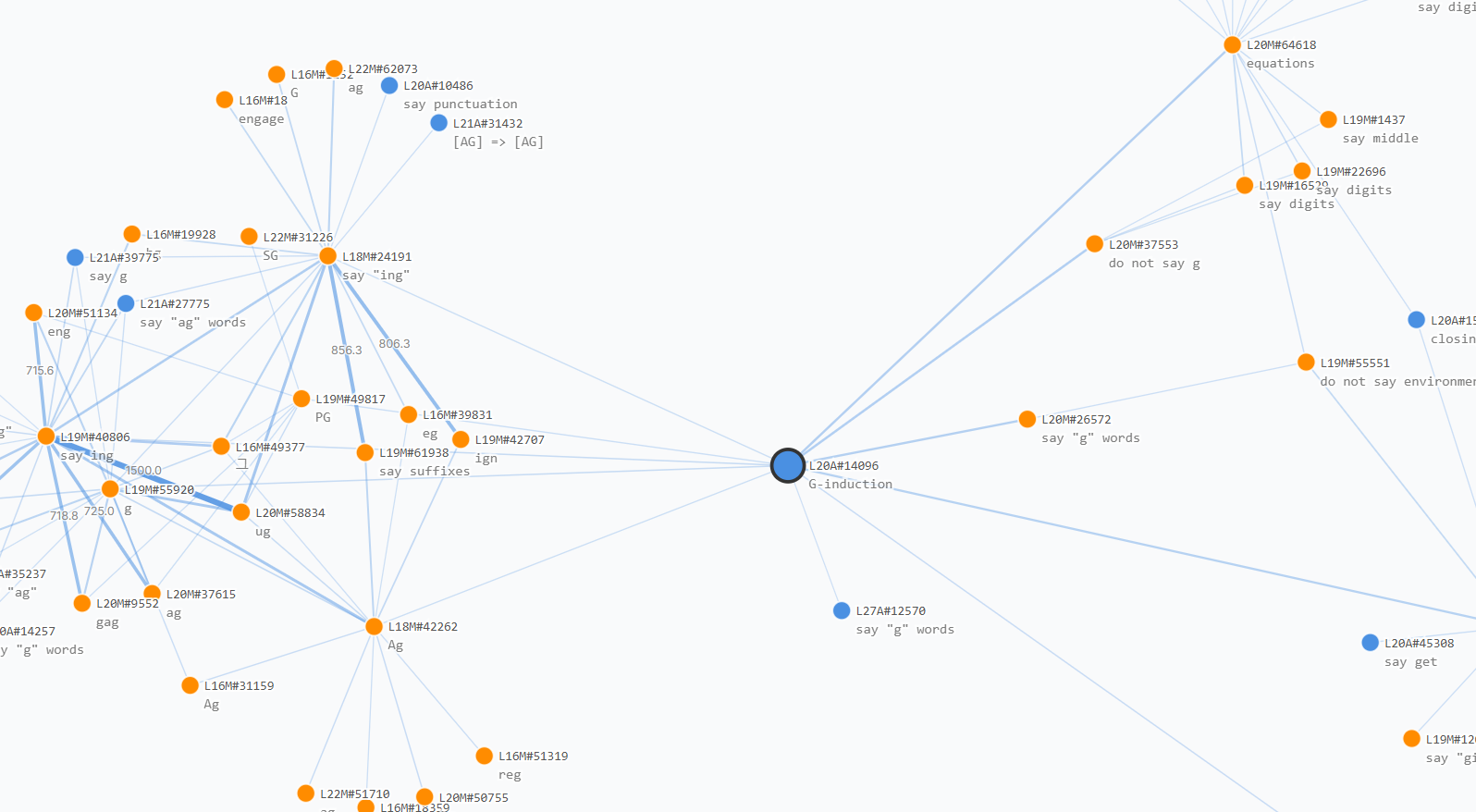
As an example, we start from a Lorsa feature at layer 20 that implements induction specific to g-related tokens (hover on top activations to see its z-pattern). The search process reveals a clear induction circuit: upstream features detect ending with g, ng, ag, and similar patterns, which feed into the induction head. Downstream, the circuit connects to features predicting g or G, as well as a number of confidence regulation features^[32] like suppressing g. The resulting global circuit is shown below.

The raw circuit produced by this search process can be quite information dense and difficult to interpret. To make them more digestible, we apply a simple pruning strategy: we remove edges below a threshold strength and filter out standalone nodes. The interactive visualization below allows exploration of these pruned atlases with adjustable edge strength thresholds.

We provide several additional global circuits seeded from other features in the model (select seed feature in the dropdown menu). For instance, starting from an Annoyance feature, we find it activated by a number of feature clusters like 怒 (anger), 不屑 (scorn), holding grudges, and had enough.

It feels like we are closer than ever to discovering the underlying global connections that explain general model behavior. We hopefully expect to see more beautiful structures (e.g. motifs and structural phenomena^[33]) in the underlying model along this direction. However, several obstacles remain.

A primary challenge is the large number of possible connections. The number of features and connections will continue to grow with the model size, which will be intractable to analyze all of them in terms of both compute and memory. Nevertheless, a sign of hope is that global connections to and from a feature are often sparse, as we observe in the global weights we studied above.

Another concern is that our current global weight analysis often resembles feature clustering rather than discovering algorithmic-like end-to-end circuits. One possible explanation is that global weights in lorsa and plt features are very short range. For example, an embedding-to-output path can have up to 56 intermediate nodes in our current setting. We might need to search through numerous turns to see a bigger picture. A potential solution is to introduce cross-layer connections (see §?).

If we manage to improve global weight analysis in these aspects, particularly in efficiency, it may become possible to reason about the model's behavior from a broader perspective and explain why the model falls short in extreme cases (e.g., adversarial examples^[2,34]). We plan to prioritize this direction in the near future.

Evaluation

In this section, we evaluate the effectiveness of the trained CRM and the attribution graphs derived from it. Following the evaluation framework proposed by Ameisen et al.^[8], we assess performance along three dimensions:

• Interpretability: We evaluate feature interpretability through automated scoring and assess the quality of the replacement layers by measuring reconstruction fidelity.
• Sufficiency: We quantify sufficiency using replacement score and completeness score as metrics to measure the proportion of error nodes in the circuit and the influence of these nodes on the final logits, quantitatively measuring how well attribution graphs capture model behavior.
• Mechanistic Faithfulness: We perform matched perturbation experiments on both attribution graphs and the original model, measuring whether interventions on feature activations produce consistent downstream effects—i.e., whether the attribution graph accurately predicts the causal consequences of perturbations in the original model.

Prior to presenting our results, it is important to notice that introducing Lorsas into the replacement model is a double-edged sword. While Lorsas enable understanding attention-mediated interactions, they also introduce additional approximation errors. The reconstruction fidelity of the CRM is thus additionally bounded, resulting in lower sufficiency metrics. This trade-off is quantified and discussed throughout the evaluation. As a result, we believe the addition of Lorsas fundamentally adds to the capability of the CRM despite newly introduced errors.

Replacement Layers Evaluation

We quantitatively assess the quality of the trained replacement layers by measuring normalized reconstruction error and explained variance. These metrics characterize how accurately the replacement layers approximate the computations of the original model components.

We also compare the reconstruction error of Lorsa and MHSA across sparsity levels. As a baseline, we control MHSA sparsity by applying AbsTopK to its concatenated \mathbf{z} vector, retaining the K channels with the largest absolute activations, analogous to the approach in §?. Lorsa achieves lower reconstruction error than MHSA even at twice the sparsity.

Attribution Graph Evaluation

Due to computational constraints, all experiments in this subsection are conducted with 8× expansion replacement models.

Computing Indirect Influence Matrix

Measuring the sufficiency and faithfulness of our replacement model depends on the indirect effect^[35,36,37], which describes the overall causal effect of an upstream node on a downstream node through all possible paths.

Indirect effect can be derived from the direct effect by iteratively aggregating paths of increasing lengths (mediated by more intermediate nodes). Starting from the attribution graph A \in \mathbb{R}^{N \times N} described in §?, where N is the number of nodes in the graph, and A_{ji} represents the direct contribution from node i to node j, we first preprocess it to get the normalized direct effect\hat{A}_{ji} = \frac{|A_{ji}|}{\sum_{k=1}^N |A_{jk}|},

where we rescale direct effect towards any target node to be all positive and sum up to 1. Indirect effect is then computed as:

Each term \hat{A}^k accumulates all k-hop paths, weighted by the product of edge weights along each path. The entry B_{ji} thus encodes all indirect influence that node i exerts on node j through paths of all lengths.

In practice, a complete attribution graph faithful to our replacement model still contains hundreds of thousands of nodes, making it intractable either to compute the complete attribution graph in adjacency matrix A or to compute the indirect influence matrix B from such a large A. We therefore adopt a greedy approximation to reduce the total node number: beginning from a subgraph containing only the logit nodes, we iteratively expand the subgraph by selecting, at each step, the node that maximizes influence on the current frontier. This procedure terminates once a predefined node budget is reached, yielding a compact subgraph that preserves the most influential pathways.

Sufficiency

In this subsection, we assess the sufficiency of the attribution graphs using two metrics proposed by Ameisen et al.^[8]: the graph replacement score, which captures how completely the graph traces information flow from embedding nodes to logits, and the graph completeness score, which quantifies the proportion of each node's indirect influence attributable to features rather than error nodes.A comparison of these scores between CRM and Transcoder-only replacement model illustrates how Lorsas affect the extent to which the attribution graphs suffice to explain model behavior.

For an attribution graph with \mathcal{N} nodes, we denote the sets of embedding nodes, feature nodes, and error nodes as \mathcal{E}, \mathcal{F}, and \mathcal{R}, respectively. The replacement score is defined as: S_{\text{r}} = \frac{\sum_{i \in \mathcal{E}} B_{\text{logit}, i}}{\sum_{i \in \mathcal{E} \cup \mathcal{R}} B_{\text{logit}, i}}.A higher replacement score indicates that the reconstruction error introduced by the graph has less actual impact on the output logits. The completeness score is defined as:S_{\text{c}} = \frac{\sum_{j \in \mathcal{N}} \left(1 - \sum_{i \in \mathcal{R}} \hat{A}_{ji}\right) B_{\text{logit}, j}}{\sum_{i \in \mathcal{N}} B_{\text{logit}, i}}.A higher completeness score indicates that, for the most influential feature nodes, a greater proportion of their indirect influence originate from features or embeddings rather than error nodes.

As expected, the CRM consistently yields a strictly lower replacement score than the Transcoder-only replacement model under the same node budget, since Lorsas introduce additional error nodes into the attribution graph, increasing the proportion of error-to-logit paths. Notably, however, we observe that this gap scales down: as the node budget and Top-K of CRM increase, the replacement score approaches that of the Transcoder-only replacement model, suggesting that the impact of these additional error nodes can be mitigated by training CRMs with larger dictionary sizes or lower sparsity.

Moreover, the CRM consistently achieves comparable or higher completeness scores than the Transcoder-only model under the same setting. We attribute this to Lorsas decomposing cross-token information flow into finer-grained paths, effectively replacing direct error-to-feature edges across tokens in Transcoder-only attribution graph with intermediate Lorsa feature nodes that better account for the sources of target feature node's indirect influence.

Mechanistic Faithfulness

Attribution graphs capture the internal mechanisms of the CRM, which, due to the reconstruction errors introduced by Transcoders and Lorsas, may deviate from the behavior of the underlying model. It is therefore essential to verify that the replacement model remains faithful to the original. Following Ameisen et al.^[8], we conduct three kinds of validation experiments to comprehensively assess whether both the replacement model and its derived attribution graphs faithfully reflect the underlying model's mechanisms.

Validating Indirect Influence within Attribution Graph

We first assess whether the influence metrics derived from the attribution graph accurately predict the causal impact of feature ablation on the underlying model's output. Specifically, for each ablated feature i, we measure the KL divergence between the original and ablated output logits as ground truth, and compute the Spearman correlation between the KL divergence values and the feature's direct influence \hat{A}_{\text{logits}, i} and indirect influence B_{\text{logits}, i}, using absolute feature activation as a baseline.

We construct attribution graphs from 100 prompts and, for each graph, individually ablate each active feature to compute the Spearman correlation. Indirect influence correlates most strongly with causal impact, followed by direct influence, with both substantially outperforming the feature activation. The correlation decreases slightly with larger Top-K, likely due to the inclusion of many low-influence features that introduce noise into the computation. As a result, it shows that "important" features indicated by our attribution graphs are highly consistent with those of the actual model behavior.

While the previous experiment validates influence at a global level from features to logits, we further examine at a finer granularity whether the indirect influence between individual feature pairs faithfully reflects the mechanisms of the underlying model.Using the same 100 prompts, we construct attribution graphs and identify the 512 features with the greatest influence on the logits in each graph. For each such feature, we ablate it and measure the resulting changes in activation of downstream features within 3 layers, computing the Pearson correlation between these changes and the corresponding indirect influence scores. We observe Pearson correlations of at least 0.62 in CRM across different sparsity settings, indicating that the graph faithfully captures the causal structure of the underlying model not only globally but also at the level of individual feature interactions.

Figures below show results from three randomly sampled examples, illustrating how well the pairwise feature influence predicts actual activation changes. Only a few points exhibit low predicted values but high actual values, confirming that the graph-based indirect influence reliably captures the actual effects between features.

Evaluating Faithfulness of CRM

To assess the overall mechanistic fidelity of the CRM, we introduce perturbations at an upstream layer and compare the resulting downstream effects in the underlying model with those propagated through the CRM. The degree of agreement between these two pathways indicates how faithfully the CRM captures the underlying model's internal mechanisms.

In these experiments, we freeze the error nodes in the replacement models, ensuring that both the CRM and the Transcoder-only replacement model match the underlying model's behavior exactly prior to perturbation. We consider three categories of perturbation vectors applied to the residual stream at a designated intervention layer:

• Encoder directions: For an active feature at the intervention layer, we add its encoder vector, scaled to increase the feature's activation by 0.1, to the residual stream.
• Random directions: As a control, we apply a random rotation to the scaled encoder vector above before adding it to the residual stream.
• Upstream features: We increase the activation of an active feature at an upstream layer by 0.1 and propagate through the replacement model to the intervention layer. The resulting change in the residual stream serves as the perturbation vector.

For each perturbation type, we run forward passes through both the underlying model and the replacement model, and at every layer beyond the intervention point, compute the perturbation effect — the difference between the perturbed and baseline residual streams. We then measure the cosine similarity and normalized MSE between the perturbation effects of the two models. For the encoder-direction and random-direction experiments, we sample 512 active features per layer; for the upstream-feature experiments, we sample 512 active features each from layer 1 and layer 14 as perturbation sources.

As shown in the bottom row, the CRM(K=64) maintains high cosine similarity across perturbation types and intervention layers. For encoder and random directions, fidelity decreases at higher layers, while for upstream features the trend is reversed, possibly reflecting shifts in the model's internal activation distribution across layers.

Overall, the CRM and the Transcoder-only replacement model exhibit comparable perturbation fidelity, indicating that the introduction of Lorsas does not significantly compromise mechanistic faithfulness. The CRM shows slightly lower fidelity near the intervention point, but this gap narrows at downstream layers, likely because downstream Lorsas can capture shifting attention patterns despite some reconstruction error, while the Transcoder-only replacement model relies on frozen attention patterns.

Related Work

Sparse Dictionary Learning

Interpretable units are the fundamental building blocks of mechanistic interpretability and circuit tracing. Sparse Dictionary Learning has emerged as a principled approach for decomposing neural network activations into sparse features, with interpretability superior to natural units like neurons and attention heads.

Despite its distant origin^[38], sparse dictionary learning has recently gained momentum through the establishment of Superposition Hypothesis^[2,39,1], which suggests that a neural network represents more features than it has neurons. Building on this hypothesis, Sparse Autoencoders (SAEs)^[3,4] have been developed to disentangle sparse features from the natural superposition in the neural network activations. Methodological improvements on SAEs have been continuously made to tackle the unique challenges in sparse training ^{[12,13,14,40]}. SAEs have also proven their ability to extract features from various internal locations^[41,42,43], from different model architectures^[44,45] and from frontier models^[12,46]. Still, outstanding limitations and challenges remain in the performance and soundness of SAE-based feature extraction^{[47,48,49,50,51]}.

One restriction of SAEs is that they learn features from a transient, isolated point of the model, make it difficult to study the interaction between features and ensure its faithfulness. Several architecutural variants have been proposed to address this limitation. Transcoders^[6,7] employ an architecture identical to SAEs, but learn to predict MLP layer outputs from their inputs, bridging over the non-linearity in MLPs. Similarly, Lorsa^[9] sparsifies MHSA to disentangle attention superposition, allowing sparse feature connections passing through attention layer. Crosscoders^[52,53,54] employ multiple parallel encoders and decoders and a unified feature space to resolve superposition among different activation spaces, either cross-layer^[52] or cross-model^{[52,53,54,55]}. Cross-layer Transcoders (CLTs)^[8] follow an architecture similar to weakly causal crosscoders, but further decouple input and output spaces, allowing for simultaneous sparsification of all MLP computations while tackling cross-layer superposition.

Circuit Discovery

Circuit Discovery methods aim to uncover the causal dependencies between components of the model. Following the definition of Olah et al. (2020)^[56], a circuit is a subgraph of the model's full computation graph (a directed acyclic graph) that partially represents the model's computation under certain tasks. Nodes of the graph represent model components (e.g. neurons, attention heads, etc.) and edges mediate the influence between them. Recent advances in circuit discovery can be roughly categorized into two categories: improvements on proper elements serving as nodes (circuit units) and improvements on how to find the nodes and edges (tracing methodology).

Improvements on Circuit Units

Circuit units are the fundamental building blocks of circuit discovery. Whether the units are understandable for human is crucial for whether the whole circuits are interpretable. Early circuit discovery methods (often referred as variants of attribution or information flow, since they do not provide explicit graph structure) primarily focused on natural units of the neural network. Researchers have attempted to highlight relevant parts of the input (typically image) in CNNs using saliency maps before mechanistic interpretability has been developed^{[57,58,59,60,61,62,63]}, where the units are directly pixels or regions in the input images. Methodologies then advanced to intermediate model components, including neurons^{[64,23,65,66]} and attention heads^[67,68,69], until recently when sparse dictionary learning methods have prevailed and sparse features become the dominant units for circuit discovery^[10,37,6,70]. Transcoder features and CLT features soon followed to enable inherent perception of model computation and allow for more robust and input-invariant circuit discovery^[7,6,8].

Improvements on Tracing Methodology

Another important direction of circuit discovery concerns how to trace important nodes and compute faithful dependencies between them. Most of the existing approaches fall into either of the following two groups: intervention-based or attribution-based.

Intervention-based methods intervene on the model, typically by changing the input or intermediate activations, and observe the downstream effects. Activation Patching (a.k.a. causal tracing, casual mediation) is the prevalent paradigm^[36], which runs the model on input A, replaces (patches) an activation with that same activation on input B, and sees how much that shifts the answer from A to B. This paradigm has been widely applied in interpretability studies^{[71,72,73,74]}. Meng et al. (2022)^[75] uses similar strategy to locate factual associations, and extends it to also edit the internal information to fix mistakes. Wang et al. (2023)^[68] develops Path Patching, which enables path-based intervention and applies it to the Indirect Object Identification task. Conmy et al. (2023)^[76] automates activation patching with a recursive patching procedure.

Attribution-based methods use attribution scores to guide the tracing process, which are the first-order Taylor expansion terms. Unlike intervention-based methods, attribution-based methods do not require separate forward passes for each interested component, but only a backward pass to obtain all the gradients.

Early interpretability studies on CNN use saliency maps, of which the form is identical to attribution scores. Inspired by patching methods, Nanda (2023)^[77] introduces Attribution Patching, which still focuses on patching from a clean run to a corrupted run, but uses attribution scores to find important components, with a total of 2 forward passes and 1 backward pass. Syed et al. (2024)^[78] finds its performance is superior to automated activation patching methods. Several works follow this paradigm to improve the gradient approximation^{[79,80,81,82]}. Marks et al. (2025)^[37] extends attribution patching to SAE features and uses integrated gradients for better approximation. Ge et al. (2024)^[6] employs transcoders and separates OV and QK circuits to keep the computational graph linear. Kamath et al. (2025)^[30] follows up to trace attentional computation in a more systematic way by checkpointing attention paths. Ameisen et al. (2025)^[8] proposes CLT based attribution graphs for a complete understanding of the model's computation for a single prompt. It is worth noting that when studying linear effects^[6,8], the attribution scores are identical to simple input decompositions (i.e. W x = \sum_i W x_i)

Discussion

Alternative Approaches to Complete Replacement Models

With a CRM, we can break down attention and MLP circuits with sparse dictionary learning methods to identify the underlying features. Introduction of attention replacement layers also implicitly solves the problem of exponential growth of attention mediated paths by injecting lorsa features into long-range feature-feature interactions.

An alternative approach introduced in Kamath et al.^[30] is to "checkpoint" attention-mediated paths by training SAEs in the residual stream at each layer and computing gradient attributions between features at adjacent layers. This forces each edge in the attribution graph to be mediated only by attention head paths of length 1, effectively cutting off longer attention-mediated paths. Our CRM achieves a similar effect: all computational paths start from a source node, pass through the residual stream (where only layernorm and lorsa attention patterns are applied), and end at a target node.

This is similar to our approach. Both methods cut off the gradient flows of attention-mediated feature-feature interactions. However, checkpointing with residual stream SAEs still cannot tackle §?—heads in the underlying model cannot be independently understood and may collectively represent some computation.

Dimensionality Collapse in Attention Outputs

Attention outputs exhibit a remarkably strong low-rank structure: approximately 60% of directions account for 99% of variance^[83]. This dimensionality collapse is fundamental to both the reconstruction quality and interpretability of attention SAEs and Lorsa layers.

Without proper initialization strategies that align feature directions with the active subspace of activations, attention replacement layers suffer from high rates of dead features and poor reconstruction fidelity. This would result in weak attention replacement layers that fail to capture the underlying attention mechanisms, ultimately preventing the construction of effective complete replacement models capable of meaningful circuit tracing and interpretability analysis.

As noted in Kamath et al.^[30], attention SAEs and attention replacement models that fail to account for this structure accumulate reconstruction error in the residual stream across layers. This leads to attributions dominated by error nodes rather than interpretable features.

Architecture Preserving Principle

The architecture-preserving principle we adopt for Lorsa layers enables CRMs to adapt to any modern transformer architecture. Most improvements to multi-head self-attention (MHSA) can be directly adapted to Lorsas, preserving the underlying architectural choices such as causal masking, attention scaling, rotary embeddings, grouped query attention, and QK-layernorm. This universality means that as transformer architectures evolve, our replacement methodology can seamlessly incorporate these advances without fundamental redesign.

However, one architectural consideration remains open for future work: GLU-based MLPs. We do not use a gate mechanism for transcoders in this work, but incorporating gates might better capture the bilinear nature of modern GLU MLPs. However, gates introduce non-linearity that could complicate attribution tracing. To maintain a linear attribution graph, we might need to detach gradients for gate activations, effectively treating them as constants during attribution computation. We leave this investigation for future work.

Inhibition and Exclusion Methods

Attribution graphs often fail to capture complete mechanistic stories, particularly when models rely on inhibition or exclusion mechanisms rather than direct positive pathways. Consider a Python error type inference task:

>>> def func(a, b): return a + b
>>> func(1)
Traceback (most recent call last):
  File "<stdin>", line 1, in <module>

The model assigns 100% probability to the correct answer, TypeError. However, attribution analysis reveals only features that enhance logits for all Python error types uniformly. There are no specific paths explaining why TypeError stands out among the alternatives.

A plausible explanation is that the model first learns to generate an error type token, then inhibits other error types, leaving TypeError as the remaining option. This inhibition-based mechanism operates through negative contributions that attribution graphs struggle to capture. Understanding such cases may require new tools that explicitly account for model exclusion and inhibition dynamics.

TODO: NDAG why not D?

Open Source Replacement Models

Cross Layer Replacement Models

Future Work